2025-04-07 lecture 18

For bandlimited graphon signals, we should be able to show convergence in the node domain!

Convergence of bandlimited signals in the node domain

Theorem

Let $(G_{n}, X_{n}) \to (W, X)$ with $c -$ bandlimited $(W, X)$ . Let $H (G_{n}) = \sum_{k = 0}^{K - 1} h_{k} (\frac{A_{n}}{n})^{k}$ be a sequence of [[graph convolution]] that share coefficients with [[graphon convolution]] $T_{H} = \sum_{k = 0}^{K - 1} h_{k} T_{W}^{(k)}$ . Then

(G_{n}, Y_{n}) \to (W, Y)

Where $Y_{n}$ and $Y$ are the graph and [[graphon convolution]] outputs respectively.

Recall that our definition of a [[convergent sequence of graph signals]] compares the [[induced graphon signal]] and the limiting [[graphon signal]] to see if they converse in an

L_{2}

way.

Proof

${\hat{Y}}_{n} \to Y$ follows ${\hat{X}}_{n} \to \hat{X}$ conbined with $\hat{H} (G_{n}) \to {\hat{T}}_{H} (W)$ . Since $X$ is bandlimited, so is $Y$ because both graph convolutions and iGFT converges to the iWFT. $◼$

See [[graph convolutions of bandlimited signals converge to the graphon convolution]]

Our first result for convergence for graphon signals is restrictive though, since we require that {as||the signal is bandlimited||restriction} and {ha||graphons have infinite-dimensional spectra||why restrictive}.

Can we get a better result? Can we generalize to arbitrary convergent graph signals?

set-up for solution

To show convergence of filters for general signals (not only bandlimited), we instead restrict {as||the filters||what restrict} to {ha||be Lipschitz||restriction}.

Lipschitz graphon filters

Let $T_{H}$ be a graphon filter. $T_{H}$ is a Lipschitz graphon filter if it has Lipschitz spectral response. ie, it

| h (λ_{1}) - h (λ_{2}) | \leq L | λ_{1} - λ_{2} | \forall λ_{1}, λ_{2} \in [- 1, 1]

This upper bounds the magnitude of the first derivative on the interval $[- 1, 1]$

Note

In this statement, our $h$ are arbitrary analytic functions. However, in practice, these will be polynomials

On the real line, polynomials are not Lipschitz. However, in a bounded interval, we can always find a Lipschitz constant.

We consider general analytic filters $h (λ)$ with Lipschitz constant $L$ (both for generality and to avoid dependence on the polynomial degree $k$ which gives us better/tighter bounds)

Improved/more general version

Aside: this is a LONG proof (longest in the class probably). The theorem is basically the same as the one above, but without the bandlimited assumption.

Theorem

Let $(G_{n}, X_{n}) \to (W, X)$ .

Let

H (G_{n}) = \sum_{k = 0}^{K - 1} h_{k} (\frac{A_{n}}{n})^{k}

be a sequence of [[graph convolution]] that share coefficients with [[graphon convolution]]

T_{H} = \sum_{k = 0}^{K - 1} h_{k} T_{W}^{(k)}

where

h (λ)

is a [[Lipschitz graphon filter]]. Then

Proof

Note

We want to show the outputs on the graph convolutions converge in the "[[induced graphon signal]]" sense to the outputs of the [[graphon convolution]]

ie, want to show $| | Y_{n} - Y | |_{2} \to 0$ where $Y_{n}$ is the [[induced graphon signal]] for $Y_{n}$ .

WLOG, we assume that $| h (λ) | \leq 1 \forall λ \in [- 1, 1]$ . We have

Y = \sum_{j \in Z ∖ {0}} h (λ_{j}) {\hat{X}}_{j} φ_{j} and Y_{n} = \sum_{j \in Z ∖ {0}} h (λ_{j}^{(n)}) [{\hat{X}}_{n}]_{j} φ_{j}^{(n)}

note on notation

$λ_{j}, X_{j}, φ_{j}$ are the eigenvalues, eigenfunctions of the eigenvectors of the graphs in the sequence of convergent graphs and convergent graph signals.

Define an partitioning index set $C$ such that

{\begin{cases} j \in C & = {i s.t. | λ_{i} | \geq c} \\ j \notin C & = {i s.t. | λ_{i} | < c} \end{cases} where c = \frac{1 - | h_{0} |}{L (2 | | X | | ϵ^{- 1} + 1)}

Where we fix some $ϵ > 0$ , $h_{0} = h (0)$ , and $L$ is the Lipschitz constant. We can choose $ϵ$ such that $c = k \forall k \in [- 1, 1]$ . Further, note that this creates a set of bandlimited components ( $C$ ) and non-bandlimited components ( $C^{c}$ ) of the signal.

Then, by the [[triangle inequality]], we have

\begin{aligned} | | Y - Y_{n} | | & = | | \sum_{j \in Z ∖ {0}} h (λ_{j}) {\hat{X}}_{j} φ_{j} - \sum_{j \in Z ∖ {0}} h (λ_{j}^{(n)}) [{\hat{X}}_{n}]_{j} φ_{j}^{(n)} | | \\ \leq | | \sum_{j \in C} h (λ_{j} {\hat{X}}_{j} φ_{j}) - \sum_{j \in C} h (λ_{j}^{(n)}) [{\hat{X}}_{n}]_{j} φ_{j}^{(n)} | | (⋆^{1}) \\ + | | \sum_{j \notin C} h (λ_{j} {\hat{X}}_{j} φ_{j}) - \sum_{j \notin C} h (λ_{j}^{(n)}) [{\hat{X}}_{n}]_{j} φ_{j}^{(n)} | | (⋆^{2}) \end{aligned}

And we can bound $(⋆^{1})$ and $(⋆^{2})$ individually.

It is very easy to bound $(⋆^{1})$ , since this is equivalent to filter applications to a bandlimited $X$ with bandwith $c$ . Thus, $(⋆^{1})$ vanishes as a direct applications of the previous result ([[bandlimited convergent graph signals converge in the fourier domain]]) to this expression.

For $(⋆^{2})$ , we note that

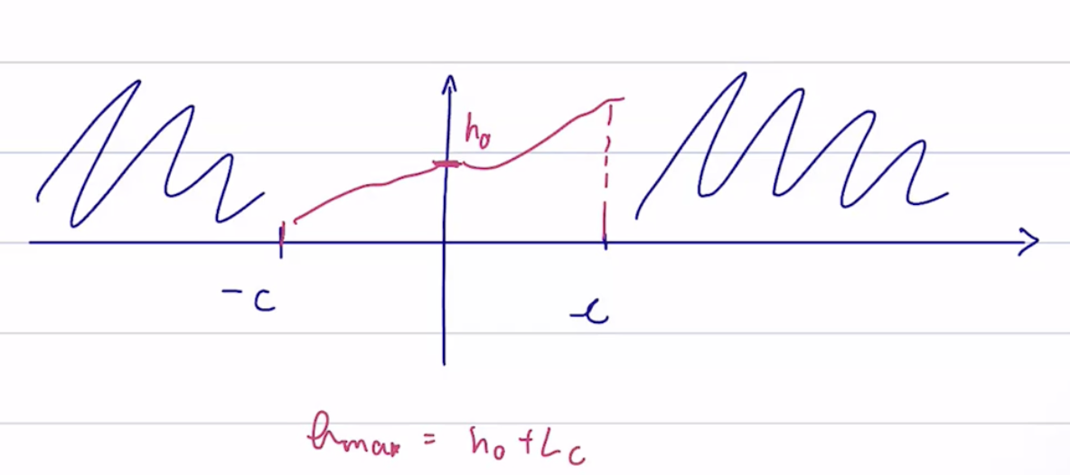
h_{0} - L c \leq h (λ_{j}) \leq h_{0} + L c \forall j \notin C

Illustration

We don't care about the spectral intervals $(- \infty, - c]$ and $[c, \infty)$ since they are covered by $(⋆^{1})$ . Since $h (λ)$ is $L$ -lipschitz, the maximum value the function can change between $0$ and $c$ is $L c$ .

Then we can write

\begin{aligned} (⋆^{2}) & = | | \sum_{j \notin C} h (λ_{j} {\hat{X}}_{j} φ_{j}) - \sum_{j \notin C} h (λ_{j}^{(n)}) [{\hat{X}}_{n}]_{j} φ_{j}^{(n)} | | \\ \leq (h_{0} + L c) | | \sum_{j \notin C} h (λ_{j} {\hat{X}}_{j} φ_{j}) - \sum_{j \notin C} h (λ_{j}^{(n)}) [{\hat{X}}_{n}]_{j} φ_{j}^{(n)} | | \\ \leq \underset{(⋆^{3})}{\underset{⏟}{h_{0} | | \sum_{j \notin C} {\hat{X}}_{j} φ_{j} - [{\hat{X}}_{n}]_{j} φ_{j}^{(n)} | |}} + \underset{(*) \leq L c | | X | |}{\underset{⏟}{L c | | \sum_{j \notin C} {\hat{X}}_{j} φ_{j} | |}} + \underset{(⋆^{4})}{\underset{⏟}{L c | | \sum_{j \notin C} [{\hat{X}}_{n}]_{j} φ_{j}^{(n)} | |}} \end{aligned}

We can see $(*)$ follows since $\sum_{j \notin C} {\hat{X}}_{j} φ_{j}$ is a portion of graphon signal $X = \sum_{j \in Z ∖ {0}} {\hat{X}}_{j} φ_{j}$ . And so, we can upper bound the norm of the portion of the signal by the norm of the entire signal.

Now, we need to bound $(⋆^{3})$ and $(⋆^{4})$ .

Note that we can write

(⋆^{†}) \sum_{j \notin C} [{\hat{X}}_{n}]_{j} φ_{j}^{(n)} = X_{n} - \sum_{j \in C} [{\hat{X}}_{n}]_{j} φ_{j}^{(n)}

We can do this because the $φ$ form an orthonormal spectral theorem).

For $(⋆^{3})$ , by writing both the [[induced graphon signal]] and the limiting [[graphon signal]] in terms of the identity $(⋆^{†})$ , we can get

\begin{aligned} | | \sum_{j \notin C} {\hat{X}}_{j} φ_{j} - [{\hat{X}}_{n}]_{j} φ_{j}^{(n)} | | & = | | (X - \sum_{j \in C} {\hat{X}}_{j} φ_{j}) - (X_{n} - \sum_{j \in C} [{\hat{X}}_{n}]_{j} φ_{j}^{(n)}) | | \\ \leq \underset{X_{n} \to X}{\underset{⏟}{| | X - X_{n} | |}} + \underset{converges (bandlimited signal)}{\underset{⏟}{| | \sum_{j \in C} {\hat{X}}_{j} φ_{j} - [{\hat{X}}_{n}]_{j} φ_{j}^{(n)} | |}} \\ < ϵ \end{aligned}

Where $ϵ$ is the same one we fixed above. Since both RHS terms converge (the first is from our initial conditions, the second one is again a direct application of bandlimited convergence), we are done for $(⋆^{3})$ .

Finally, for $(⋆^{4})$ ,

\begin{aligned} | | \sum_{j \notin C} [{\hat{X}}_{n}]_{j} φ_{j}^{(n)} | | & = | | X_{n} - \sum_{j \in C} [{\hat{X}}_{n}]_{j} φ_{j}^{(n)} + X - X | | \\ \leq \underset{X_{n} \to X}{\underset{⏟}{| | X_{n} - X | |}} + \underset{converges (bandlimited)}{\underset{⏟}{| | \sum_{j \in C} [{\hat{X}}_{n}]_{j} φ_{j}^{(n)} - {\hat{X}}_{j} φ_{j} | |}} + \underset{\leq | | X | |}{\underset{⏟}{| | \sum_{j \notin C} {\hat{X}}_{j} φ_{j} | |}} \\ < ϵ + | | X | | \end{aligned}

Thus we get that

\begin{aligned} (⋆^{2}) & = | | \sum_{j \notin C} h (λ_{j} {\hat{X}}_{j} φ_{j}) - \sum_{j \notin C} h (λ_{j}^{(n)}) [{\hat{X}}_{n}]_{j} φ_{j}^{(n)} | | \\ \leq L c | | X | | + h_{0} ϵ + L c (ϵ + | | X | |) \\ < \tilde{ϵ} \end{aligned}

for all $n > N_{ϵ}$

see [[lipschitz graph convolutions of graph signals converge to lipschitz graphon filters]]

Summary

For node-domain convergence, we first saw that graphons have infinite-dimensional spectra, this can be quite strict and therefore not super useful. Instead, we replaced the bandlimited assumption with a Lipschitz continuity requirement.

It was difficult to show convergence for the GFT for spectral components associated with eigenvalues close to

0

(see conjecture 1 from Lecture 17). This is why we showed instead that [[bandlimited convergent graph signals converge in the fourier domain]].

Here, the same thing happens because accumulate at 0. The Lipschitz continuity addresses this by ensuring all spectral components near 0 are amplified in an increasingly "similar" way. We can see this by looking at how we defined

c

in the proof:

Transferability of Graph Convolutions and GNNs

The asymptotic convergence of the lipschitz graph filters reveals an important tradeoff between convergence/transferability and discriminability. We can compare this to the [[stability-discriminability tradeoff for Lipschitz filters]].

c

-band cardinality

$c$ -band cardinality of a graphon eigenvalues with magnitude greater than $c$

n_{c} (W) = | {λ_{i} : | λ_{i} | > c} |

Note that this quantity is finite since the [[graphon shift operator eigenvalues]] accumulate only at 0.

c

-eigenvalue margin

The $c$ -eigenvalue margin of graphons $W$ and $W^{'}$ is the minimum difference between and [[eigenvalue]] of $W^{'}$ outside of the $c$ band and an eigenvalue of $W$ :

δ_{c} (W, W^{'}) = min_{i \neq j} {| λ_{i} (T_{W^{'}}) - λ_{j} (T_{W}) | : | λ_{i} (T_{W^{'}}) | \geq c}

Non-asymptotic convergence of graph convolutions

Theorem

Let $(G_{n}, X_{n}) \sim (W, X)$ and let graph and graphon convolutions be such that

H (G_{n}) = \sum_{k = 0}^{\infty} h_{k} {(\frac{A_{n}}{n})}^{k} and T_{H} = \sum_{k = 0}^{\infty} h_{k} T_{W}^{k}

Further, assume

$| | X | | \leq 1$ (WLOG)
$| h (λ) | < 1$ and $h (λ)$ is $L -$ Lipschitz in $[- 1, - c] \cup [c, 1]$ and $ℓ -$ Lipschitz in $(- c, c)$

Then we have

| | Y_{n} - Y | | \leq (L + \frac{π n_{c}}{δ_{c}}) | | T_{W} - T_{W_{n}} | | + (L c + 2) | | X - X_{n} | | + 2 ℓ c

Note

note that this bound depends on

the norm difference between the [[graphon]] and the [[induced graphon]] $| | T_{W} - T_{W_{n}} | |$
the the norm difference between the [[graphon signal]] and the [[induced graphon signal]] $| | X - X_{n} | |$

We already know that these two things converge (we've already discussed the (slow) convergence rate for $W_{n}$ in induced [[graph sequence converges if and only if the induced graphon sequence converges]]). We can bring the rates for both quantities to $O (\frac{1}{n})$ by introducing more restrictive requirements.

Here, the convergence-discriminability tradeoff is explicit. We can see that larger

L

and smaller

c

(more discriminative filters) lead to a higher error bound.

The last term

2 ℓ c

does not vanish. We can think of this as the "approximation error" that comes from the fact that the eigenvalues of the graphs converge non-uniformly (recall this conjecture).

In the finite sample regime, unless

ℓ = 0

, there is always leftover "nontransferable energy" corresponding to the spectral components with

| λ_{i} | < c

which do not converge

Review

What does the lipschitz condition achieve in [[lipschitz graph convolutions of graph signals converge to lipschitz graphon filters]]?
-?-
it ensures all spectral components near 0 are amplified in an increasingly "similar" way.

3. [[Graphon Signal Processing]]

Convergence of bandlimited signals in the node domain

set-up for solution

Improved/more general version

Transferability of Graph Convolutions and GNNs

Non-asymptotic convergence of graph convolutions

Review