2025-03-26 lecture 15

[[lecture-data]]

2. [[GNN Analyses]]

Last time, we left off defining a metric for graphs with potentially different node counts.

Let $G_{n}, G_{m}$ be graphs with $n$ and $m$ nodes respectively, with $n \neq m$ . We bring them into a common reference frame by comparing their {induced graphons} instead of attempting to compare the graphs directly.

induced graphon

Let $G_{n}$ be a graph with $n$ nodes. The graphon induced by $G_{n}$ is
$W_{n} (u, v) = \sum_{i = 1}^{n} \sum_{j = 1}^{n} A_{i j} 1 (u \in I_{i}) \cdot 1 (v \in I_{j})$
where $1$ is the indicator function and $I_{k}$ is defined as
$I_{k} = {\begin{cases} [\frac{k - 1}{n}, \frac{k}{n}) 1 \leq k \leq n - 1 \\ [\frac{n - 1}{n}, 1] k = n \end{cases}$

cut norm (kernels)

Let $W$ be a kernel in $[0, 1]^{2}$ . Its cut norm is defined as
$| | W | |_{◻} = sup_{S, T \subseteq [0, 1]} | \int \int_{S \times T} W (u, v) d u d v |$

Note

We want to use the induced graphons (recall we do this by dividing the interval $[0, 1]$ into $n$ subintervals each corresponding to a node).

However, the cut norm does not take into account {ass||permutations of the intervals $I_{k}$ ||limitation} so {has||we cannot use this norm to define our metric directly||consequence}. To take these into account, we use {hha||measure-preserving bijections on the sample space/support for the graphon $W$ (typically the unit interval) which we can think of as "permutations"||workaround}.

Cut Metric

The cut metric for two graphons (kernels) is given by
$\delta_{\square}(W,W') = \inf_{\varphi} \lvert \lvert W^{\varphi}-W' \rvert \rvert_{\square} $
Where $| | \cdot | |_{◻}$ is the [[cut norm]] and $W^{φ} (u, v) = W (φ (u), φ (v))$ and $φ$ are measure-preserving bijections (on the unit interval)

Thus, for two arbitrary graphs, we can define the cut distance:

Cut distance (arbitrary graphs)

Let $G_{n}$ and $G_{m}$ be two graphs with possibly different node counts $n$ and $m$ respectively. The cut distance is given by

δ_{◻} (G_{n}, G_{m}) = δ_{◻} (W_{n}, W_{m})

Where $W_{n}, W_{m}$ are the induced graphons of the graphs.

see [[cut distance]]

Note

We can show equivalence of right- and left- cut [[homomorphism density]] convergence with the [[cut distance]] for dense graphs.

Theorem

Sequences of graphs ${G_{n}}$ converging to [[graphon]] $W$ also converge in the [[cut norm]]:

G_{n} \to W ⟺ | | W_{n} - W | |_{◻} \to 0 as n \to \infty

Where $W_{n}$ is the [[induced graphon]] of $G_{n}$ .

see [[graph sequence converges if and only if the induced graphon sequence converges]]

In fact, to show that left and right convergence with the cut metric/[[cut norm]] as above.

Proofs are in the book Large networks and convergent graph sequences by Lavàsz (online). For the equivalence in [[homomorphism density]], see section counting and inverse counting lemmas.

Summary

This answers the question that we had last time

Question

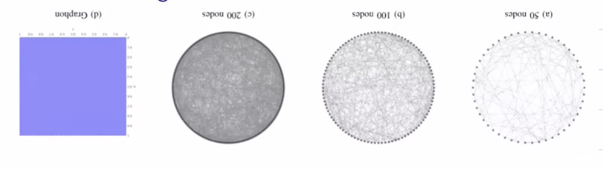
What happens when the graph grows?

Can we measure how “close” two large graphs are? ie, can we define a metric for two large graphs?

Answer

The limiting object of a [[convergent graph sequence]] is a [[graphon]]. We use the (left) [[homomorphism density]] to show this convergence.

Answer

The induced graphons.

Now, we address

Question

2. Can we prove the GNN is continuous WRT to this metric?

Relationship between the graphons

(and [[graphon distances]] which have codomain $[- 1, 1]$ )

Note

Inequality results comparing the L-p norms are for kernels that are {ass||more general than our graphons||comparison to graphon}. We want {has||the codomain to be $[- 1, 1]$ ||modification} because {hha||taking the [[cut norm]] for a difference of graphons $W - W^{'}$ gives values in this interval.||modification reason}

Let $W : [0, 1]^{2} \to [- 1, 1]$ .

Trivially:

| | W | |_{◻} \leq | | W | |_{1} \leq | | W | |_{2} \leq | | W | |_{\infty} \leq 1

Easy to see from definition of [[cut norm]] where we are essentially computing the $L_{1}$ -norm. Then we know already the rest of the inequalities.

$⟹$ convergence in $L_{p}, p \geq 1$ implies cut norm convergence

Theorem

Let $W : [0, 1]^{2} \to [- 1, 1]$ . Then

| | W | |_{◻} \overset{(1)}{\leq} | | W | |_{1} \overset{(2)}{\leq} | | W | |_{2} \overset{(3)}{\leq} | | W | |_{\infty} \overset{(4)}{\leq} 1

And convergence $L_{p}$ for $p \geq 1$ implies convergence in the [[cut norm]]

Proof

Easy to see (1) from the definition of the cut norm:

cut norm (kernels)

Let $W$ be a kernel in $[0, 1]^{2}$ . Its cut norm is defined as
$| | W | |_{◻} = sup_{S, T \subseteq [0, 1]} | \int \int_{S \times T} W (u, v) d u d v |$

This is computing the L-1 norm restricted to a subset of the nodes, so $| | W | |_{◻} \leq | | W | |_{1}$ .

(2) and (3) are a common result from functional analysis, and (4) is because of the selected codomain for $W$ .

Convergence in the [[cut norm]] follows immediately from this hierarchy.

see [[convergence in L-p implies convergence in cut norm]]

In the other direction:

| | W | |_{2, 2} \leq \sqrt{4 \cdot | | W | |_{\infty \to 1}} \leq \sqrt{16 \cdot | | W | |_{◻}}

$⟹$ [[cut norm]] convergence implies convergence in $L_{2}$

Theorem

Let $W : [0, 1]^{2} \to [- 1, 1]$ . Then

| | W | |_{2, 2} \overset{(1)}{\leq} \sqrt{4 \cdot | | W | |_{\infty \to 1}} \overset{(2)}{\leq} \sqrt{16 \cdot | | W | |_{◻}}

ie, [[cut norm]] convergence implies convergence in $L_{2}$

see [[Convergence in the cut norm implies convergence in L2]]

Proof of (2)

We first show inequality (2). Using the definition of the [[cut norm]], we have

\begin{aligned} | | W | |_{◻} & = sup_{S, T \subseteq [0, 1]} | \int \int_{S \times T} W (u, v) d u d v | \\ = sup_{f, g : [0, 1] \to [0, 1]} | \int_{0}^{1} \int_{0}^{1} W (u, v) f (u) g (v) d u d v | \\ (*) & = sup_{f, g : [0, 1] \to [0, 1]} | ⟨ T_{W} f, g ⟩ | \end{aligned}

Since we are taking the supremum, it is equivalent to taking the supremum over all $L_{\infty}$ functions $f$ and $g$ .

To get $(*)$ , we notice that $\int_{0}^{1} W (u, v) f (u) d u$ is an [[integral linear operator]] with kernel $W$ . We denote this with $T_{W}$ so that

T_{W} f (v) = \int_{0}^{1} W (u, v) f (u) d u

or equivalently that $T_{W} f = \int_{0}^{1} W (u, \cdot) f (u) d u$
We can then see that the definition becomes the absolute value of the inner product of two $L_{\infty}$ functions.

Note that $| | W | |_{\infty \to 1}$ is an induced [[operator norm]] of the [[graphon]] mapping functions from $L_{\infty}$ to $L_{1}$ .

\begin{aligned} | | W | |_{\infty \to 1} & = sup_{- 1 \leq g \leq 1} | | T_{W} g | |_{1} \\ = sup_{- 1 \leq g \leq 1} \int | T_{W} g (x) | d x \\ = sup_{- 1 \leq f, g \leq 1} ⟨ T_{W} g, f ⟩ \end{aligned}

we omit the denominator in our usual definition of the [[operator norm]] since $g$ is bounded by $- 1$ and $1$ and $g \in L_{\infty}$
We can rewrite this using $f$ to match in the definition of the $L_{1}$ norm since we are taking the supremum
For more about $L_{p}$ spaces see wikipedia (hand wavy/cursory for this class on functional analysis details)

We can then rewrite this as

\begin{aligned} | | W | |_{\infty \to 1} & = sup_{- 1 \leq f, f^{'} \leq 1, - 1 \leq g, g^{'} \leq 1} ⟨ T_{W} (g - g^{'}), f - f^{'} ⟩ \\ (* *) & \leq sup_{- 1 \leq g, f \leq 1} ⟨ T_{W} g, f ⟩ - sup_{- 1 \leq g, f^{'} \leq 1} ⟨ T_{W} g, f^{'} ⟩ + sup_{- 1 \leq g^{'}, f \leq 1} ⟨ T_{W} g^{'}, f ⟩ - sup_{- 1 \leq g^{'}, f^{'} \leq 1} ⟨ T_{W} g^{'}, f^{'} ⟩ \\ (†) & \leq 4 | | W | |_{◻} \end{aligned}

Where we get $(* *)$ by the [[triangle inequality]] and $(†)$ from the definition of $| | \cdot | |_{◻}$ .

Note that this is a loose bound!

And this gives us the desired result for (2).

Proof of (1)

Proving (1) is more involved and uses more functional analysis.

Use the Riesz-Thorin interpolation theorem for complex $L_{p}$ spaces:

| | W | |_{p \to q} \leq | | W | |_{p_{1} \to q_{0}}^{1 - θ} | | W | |_{p_{1} \to q_{1}}^{θ}

Where

$θ = min (1 - \frac{1}{p}, \frac{1}{q})$ and
$p_{0}, q_{0} \in [1, \infty)$
with $\frac{1}{p} = \frac{1 - θ}{p_{0}}$ and
$1 - \frac{1}{q} = (1 - θ) (1 - \frac{1}{q_{0}})$ and
$p_{1} = \infty, q_{1} = 1$ .

Define [[operator norm]]$$\lvert \lvert W \rvert \rvert_{\square, \mathbb{C}} = \sup_{\begin{aligned}
f,g:[0,1] &\to \mathbb{C} \\lvert \lvert f \rvert \rvert_{\infty}, \lvert \lvert g \rvert \rvert_{\infty} &≤1 \end{aligned}} \left\lvert \int {0}^1 \int^1 W(u,v) f(u) g(v) , du , dv \right\rvert $$
So for complex functions, we can see that

\begin{aligned} for complex functions | | W | |_{\infty \to 1} & = | | W | |_{◻, C} \\ \leq 2 | | W | |_{\infty \to 1} for real functions \end{aligned}

We then have

| | W | |_{p_{0} \to q_{0}} \leq | | W | |_{1 \to \infty} \leq | | W | |_{\infty} \leq 1

Since $W \leq 1$ , and this gives the desired result.

convergence in the 2 norm

idea/preview
If we have a sequence of convergent graphs that converges to a [[graphon]], then the [[graph shift operator]] (typically $A$ ) converges in an "operator sense" to the [[integral linear operator]] that we defined above $T_{W} f (v) = \int_{0}^{1} W (u, v) f (u) d u$ .

see [[graph shift operators converge to graphon shift operators]]

Takeaways

We defined [[convergent graph sequence]] converging to [[graphon]]
If two graphs belong to the same sequence, we know they are similar using the [[homomorphism density]]
Defined a metric with the cut metric to compute distances between graphs
If we have convergence in some $L_{P}$ spaces, we also have convergence in the [[cut norm]] and vice versa.
We can look at graphons as operators

can we use graphons to sample subgraphs?

Recall the question we had

Question

What if the graph is too large and I don’t have enough resources to train on it? (recall GNN forward pass is $O (L K \cdot | E |)$ where $L$ is the number of layers and $K$ is the order of the filter polynomial)

we can think of graphons as generative models as well

Example

Graphon as a limiting object for some sequence of graphs

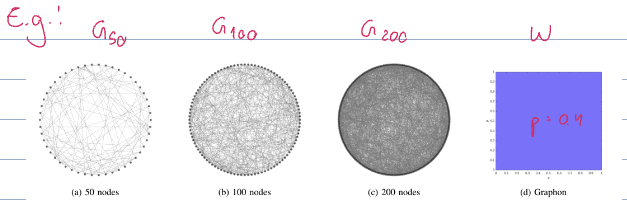
Graphon as generating object for finite graphs

options for sampling nodes and edges from graphons

[[template graph]]

see [[ways to sample graphs from graphons]]

template graph

A template graph $G_{n}$ is a way to sample a graph from a graphon. The nodes are defined by partitioning $[0, 1]$ in a grid (regular partition) in the same way we partitioned for induced graphons:

I_{k} = {\begin{cases} [\frac{k - 1}{n}, \frac{k}{n} [1 \leq k \leq n - 1 \\ [\frac{n - 1}{n}, 1] k = n \end{cases}

So that $I_{1} \cup I_{2} \cup \dots \cup I_{n} = [0, 1]$ and the node labels are $u_{j} = \frac{j - 1}{n}$ for each $j$ .

The [[adjacency matrix]] is then given as

[A_{n}]_{i j} = W (u_{i}, u_{j})

Where $W$ is the [[graphon]] that we sample from.

This is a complete, weighted graph with edge weights coming from the [[graphon]] evaluated at each node pair $(u_{i}, u_{j}) \in [0, 1]^{2}$ .

This is the simplest way to sample a graph. We can think of it as the graph sampling counterpart to inducing a graphon.

see [[template graph]]

weighted graphs

Weighted graphs are a way to sample a graph from a graphon. Each node $u_{j}$ is sampled uniformly at random from the unit interval.

The edges are then defined in the same way as a [[template graph]]

[A_{n}]_{i j} = W (u_{i}, u_{j})

see [[weighted graph (sample)]]

Def

Fully random graphs are a way to sample a graph from a graphon. Like a [[weighted graph (sample)]], the nodes are sampled uniformly from the unit interval ( $u_{i} \sim U [0, 1]$ ).

The edges are sampled as

[A_{n}]_{i j} = [A_{n}]_{j i} \sim Bernoulli (W (u_{i}, u_{j}))

So the resulting graph is undirected and unweighted .

see [[fully random graph]]

Note

Generally we are interested in the fully random graphs.

[?] could we sample the nodes randomly, then sample the edge weights from the 2D interval?

All of the graphs above converge to $W$ in some sense.

Template graphs: trivial

Theorem

Let ${G_{n}}$ be a sequence of template graphs sampled from [[graphon]] $W$ . Then $G_{n} \to W$ as $n \to \infty$ .

Proof

Trivial

The definition of template graphs is fully deterministic, so there is no randomness here. Since this is the reverse idea of thinking of graphons as graphs with uncountable number of nodes, it is easy to see that the induced graphons $W_{n}$ converge to $W$ in an $L_{2}$ way and [[convergence in L-p implies convergence in cut norm]]

see [[template graphs converge to the graphon]]

Theorem

Let ${G_{n}}$ be a sequence of weighted graphs sampled from [[graphon]] $W$ . With probability at least $1 - \exp (- \frac{n}{2 \log n})$ ,

δ_{◻} (G_{n}, W) \leq \frac{20}{\sqrt{\log n}}

Where $δ_{◻}$ is the cut metric. ie, $G_{n} \to W$ in probability.

see [[weighted sampled graphs converge to the graphon in probability]]

random

Theorem

Let ${G_{n}}$ be a sequence of "fully random" graphs sampled from [[graphon]] $W$ . With probability at least $1 - \exp (- \frac{n}{2 \log n})$ ,

δ_{◻} (G_{n}, W) \leq \frac{22}{\sqrt{\log n}}

Where $δ_{◻}$ is the cut metric. ie, $G_{n} \to W$ in probability.

see [[fully random graphs converge to the graphon in probability]]

Note

We'll look at the proofs for these later.

Tip

If a graph is too big to train on it, we can look at the [[induced graphon]] and subsample new graphs from it to train on instead.

GNN continuity

Question

How do we determine whether a GNN continuous with respect to the cut metric?

In order to transfer from small graphs to large graphs, we need continuity. In particular, we need Lipschitz continuity with a not-very-large constant.

Question

Do GNNs converge?

This question has a long answer. To start to answer it, we need to introduce graphon signals and graphon signal processing.

These are extensions of [[Graph Signals and Graph Signal Processing]]

road map

generalize up from graphs to graphons
graph convolution to [[graphon convolution]]
intuition behind why GNNs generalize well with scale
then look at bounds
- finite sampling bounds
- minimum sample sizes
- error bounds

Note

we focus a lot on information processing pipelines and GNNs, but there are also many other applications for graphons. Many people are interested in graphon estimation / the underlying distribution for some graphs.

Graphon signal

A graphon signal is defined as a function

X : [0, 1] \to R

Note

contrast this with [[graph signals]], which we defined as $x \in R^{n}$ .

Note

We focus on signals in $L_{2}$ , or "finite energy signals" $X \in L_{2} ([0, 1])$ :

\int_{0}^{1} | X (u) |^{2} d u \leq B < \infty

see [[graphon signal]]

Like a [[graphon]], a [[graphon signal]] is the limit of a [[convergent sequence of graph signals]]. Like when defining our [[cut distance]] for differently sized graphs, the [[graph signals]] may have different sizes since the dimension changes with the number of nodes $n$ . Similarly, we solve this with [[induced graphon signal]]

Induced Graphon Signal

Let $(G_{n}, X_{n})$ be a graph signal. The induced graphon signal is defined as the pair $(W_{n}, X_{n})$ where $W_{n}$ is the [[induced graphon]] and

X_{n} (u) = \sum_{i = 1}^{n} [x_{n}]_{i} 1 (u \in I_{i})

Where $1$ is the indicator function and

I_{k} = {\begin{cases} [\frac{k - 1}{n}, \frac{k}{n}) 1 \leq k \leq n - 1 \\ [\frac{n - 1}{n}, 1] k = n \end{cases}

Example

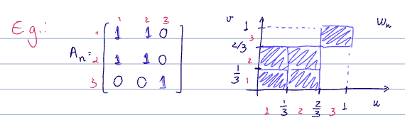
Both representations of 3-node graphs ([[induced graphon]] above and induced graphon signal below)

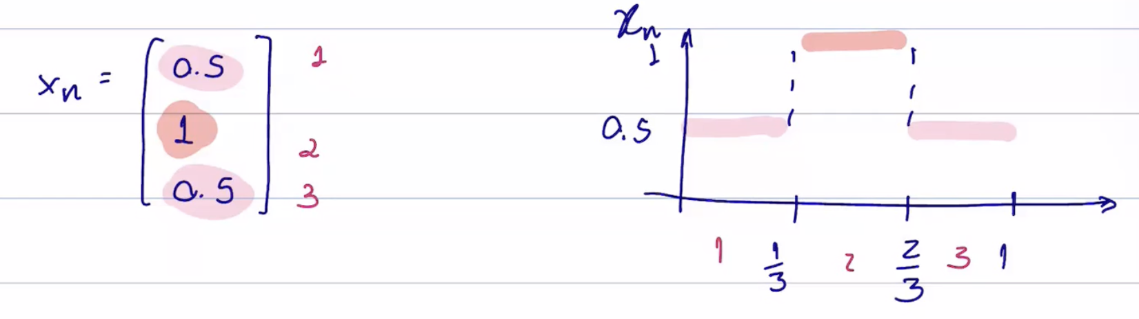
see [[induced graphon signal]]

Review

#flashcards/math/dsg

const { dateTime } = await cJS()

return function View() {
	const file = dc.useCurrentFile();
	return <p class="dv-modified">Created {dateTime.getCreated(file)}     ֍     Last Modified {dateTime.getLastMod(file)}</p>
}