2025-03-24 graphs lecture 14
[[lecture-data]]
- val acc not stable for expressivity : normal since small val set. Loss smooth
- typical for graph-level problem
- stability: 10-30% goal to see stable degrades for different models
- gnn slower than for filters
- more layers = more stable for gnn (more nonlinearities)
- discuss degradation
- Last prob
- penalize vs not penalized
- plot model 2’ vs mod 2
- 1-2 ppl
- either novel graph data/train model : 10min presentation
- research paper presentation on any modern GNN/graph DS (past 5 years): 20 min presentation
- review/discussion
Limits of Graphs
Last time, we looked at different graph perturbations and how to design stable GNNs. We saw how GNNs inherit stability from their layers and that GNNs perform better than their constituent filters because of the scattering of spectral information by the nonlinear activation function.
- What if the graph grows?
- What if the graph is too large and I don’t have enough resources to train on it? (recall GNN forward pass is
where is the number of layers and is the order of the filter polynomial)
To address problem 2 (what if the graph is too large?), we can subsample the graph with a random graph model. We will talk about this later.
Today, we turn to problem 1 (what if the graph grows?). To address this, we want to know
- Can we measure how “close” two large graphs are? ie, can we define a metric for two (large) graphs?
- If we can, then we can see if a GNN is continuous. If we can prove the GNN is continuous, then we are OK (perturbations will affect the function in a predictable way). Then,
- Can we prove the GNN is continuous WRT to this metric?
What does it mean for two graphs to be “close”? We’ll say this happens when they converge to a common limit.
defining a metric between graphs
What does it mean for graphs to be “close”?
- From a probability POV, it makes sense to say that graphs are “close” if {sampled subgraphs have similar distributions}.
- Equivalently, from a statistics POV, we say graphs are “close” if they {have similar subgraph counts (triangle counts, degrees, etc)}
To measure the subgraph counts, we can use homomorphism density. Recall from lecture 11 the definition of a graph homomorphism
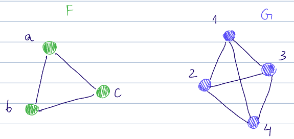
There are a few homomorphisms from
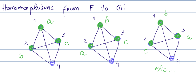
- And trivially, every permutation of
is also a homomorphism here
- And trivially, every permutation of
There are also:
and for each of the above, each permutation ofas well.
The homomorphism count
Recall also the definition for the homomorphism density:
in the example above,
This equates to the probability of sampling a triangle from
The astute reader will see that we can use the homomorphism density to compare graphs from the statistics POV of sampling. To do this, we need some subgraphs that serve as references for the types of counts we want (eg. triangles).
Let
- undirected
- unweighted
- with 1 edge per node pair
- not loopy (no self edges)
(see graph motif)
We can use this to create an idea of “closeness” for two graphs
To formalize this idea into a definition, we first need to define what a convergent graph sequence is.
Convergent graph sequences and graphons
More info from Levàsz, Chayes, Borgs, Vesztergambi starting 2008-on
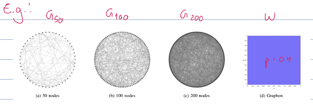
To begin, we need to define the “limit” of a sequence of graphs as the number of nodes
We call the limit of a sequence of graphs of increasing node count a {graphon}
(see graphon)
A more general definition is
where
Show that if the CDF of
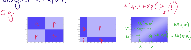
If the limit of the graph sequence
The density from a graph motif
This is the generalization of the definition of the homomorphism density
If
Erdos-Renyi with
(see graphon homomorphism density)
(see convergent graph sequence)
- This is more of a “local” idea of convergence since it checks to see if sampled subgraphs converge up to the limiting object. This is called left convergence since it deals with left homomorphism densities
and . - This is not the only way to identify a (dense) convergent graph sequence. Another definition is based on the convergence of min-cuts or right homomorphisms
and . - This is a more “global” notion of convergence that is used sometimes by graph theorists or in physics (micro-canonical ground state energy)
- Fore dense graphs, left and right convergence are equivalent (for the metric we like) without proof.
- Dense graphs are ““convex””
metric on graphs
While
We want to use a metric that is easier to calculate. Eventually, we want a distance for arbitrary graphs
same node count and labels
Let
Let
see cut norm
The cut distance will be our metric of choice in most cases.
same node count, different labels
Let
ie, we look at all possible permutations of the nodes of
different node counts
Let
To do this, we can bring them into graphon space. So we need to define graphons induced by these graphs.
Let
where
see induced graphon
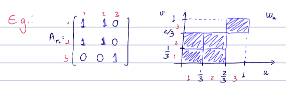
This “chops up” the axes into intervals of size
We can define both
Let
see kernel cut norm
const { dateTime } = await cJS()

return function View() {
	const file = dc.useCurrentFile();
	return <p class="dv-modified">Created {dateTime.getCreated(file)}     ֍     Last Modified {dateTime.getLastMod(file)}</p>
}