2025-03-10 graphs lecture 13

[[lecture-data]]

finish cleaning up these notes once PDF is published #class_notes/clean ➕ 2025-03-10 📅 2025-03-12 ✅ 2025-03-12

Summary

Last Time

lipschitz graph filter
Today
finish stability of GNNs

Notes PDF

1. Graph Signals and Graph Signal Processing

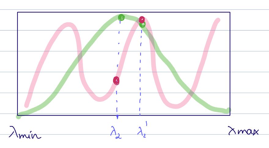
Recall the definition for an integral Lipschitz filter

integral lipschitz filter

Let $h (λ)$ be the spectral representation of a convolutional graph filter. $h (λ)$ is integral lipschitz on interval $T \subset R$ means there exists some $c \in R$ such that
$| h (λ) - h (λ^{'}) | \leq \frac{C | λ^{'} - λ |}{\frac{1}{2} | λ + λ^{'} |} \forall λ, λ^{'}$
ie, $h (λ)$ is lipschitz with a constant inversely proportional to the interval's midpoint

Letting $λ^{'} \to λ$ , we get
$λ h^{'} (λ) \leq c ⟹ h^{'} (x) \leq \frac{c}{λ} \to 0, λ \to \infty$
This means that the filter can't change for large $λ$ .

Example

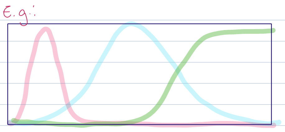
Notice that the filter becomes flat at high frequencies

At low $λ$ , they can be arbitrarily thin.
At medium $λ$ , these filters are approximately lipschitz filters.
At high $λ$ , they become flat and lose discriminability

Note

$c$ controls how discerning an integral Lipschitz filter is for frequencies at different ranges.

Stability to different graph perturbations

Recall the types of perturbations on shift operators:

Perturbation Types

We consider 3 perturbation types (first for graph convolutions, then for GNNs)

operator dilation

Let $S$ be a shift operator. We call $S^{'}$ an (operator) dilation (or scaling) if
$S^{'} = (1 + ϵ) S$
$\implies \lvert \lvert S-S' \rvert \rvert = \epsilon \lvert \lvert S \rvert \rvert $
We can interpret this as the edges being scaled by $(1 + ϵ)$ .

Additive Perturbations

Let $S$ be a matrix. $\tilde{S}$ is an additive perturbation of $S$ if
$\tilde{S} = S + E, E = \tilde{S} - S, 0 \leq | | E | | \leq ϵ$
However, this definition is problematic since it is not invariant to permutations:
$\tilde{S} = P^{T} S P ⟹ E = P^{T} S P - S$

For a graph shift operator, we define an additive perturbation modulo permutations:
$E (S, \tilde{S}) = {D : P^{T} \tilde{S} P = S + D}$
Where $P \in P$ is a permutation.

Given $\tilde{S}$ , the error is the $D$ with the smallest norm:
$\tilde{E} = \arg\min_{D \in E(S, \tilde{S})} \lvert \lvert D \rvert \rvert_{p} $
Where $| | \cdot | |_{p} = d (\cdot)$ is the operator distance modulo permutations and $| | D | |_{p} = d (S, \tilde{S})$

Unlike dilation, absolute perturbations (like the additive perturbations) do not take edge weights into account but can model changes in edge existence. This is fine for unweighted graphs, but for weighted graphs, this renders them unmeaningful. We want something that both

takes edge weights into account
can model edge additions and deletions
ie a perturbation that can combine these two benefits.

Relative Perturbations modulo permutations

$E (S, \tilde{S}) = {D : P^{T} S P = S + D S + S D, P \in P}$

given $\tilde{S}$ , the error is $E$ with the smallest norm ie

\tilde{E} = \arg min_{D \in E (S, \tilde{S})} | | D | |

ie $| | \tilde{E} | | = d (S, \tilde{S})$

where $d (\cdot)$ is the operator distance modulo permutations.

Note

dilation takes into account edge weights, but cannot model edge additions and deletions
additive perturbations can model edge additions and deletions, but do not take into account edge weights
relative perturbations take into account both edge weights and additions/deletions

see relative perturbations

stability for dilations

Theorem

Let $S^{'} = (1 + ϵ) S$ be a dilation, and consider graph convolution $H (S)$ . If $H (S)$ is a integral Lipschitz filter with constant $c$ , then

| | H (S) - H (S^{'}) | | \leq c ϵ + O (ϵ^{2})

ie, integral Lipschitz filters are stable to dilations/scalings

Proof

$\begin{aligned} H (S^{'}) - H (S) & = \sum_{k = 0}^{\infty} S^{' k} - \sum_{k = 0}^{\infty} S^{k} \\ S^{'} = (1 + ϵ) S ⟹ H (S^{'}) - H (S) & = \sum_{k = 0}^{\infty} h_{k} ((1 + ϵ^{k}) S^{k} - S^{k}) \end{aligned}$

Via binomial expansion, we have

\begin{aligned} (1 + ϵ)^{k} & = \sum_{i = 0}^{\infty} (\binom{k}{i}) ϵ^{k} \\ = 1 + k ϵ + o_{k} (ϵ) \end{aligned}

Recall that $o_{k} (ϵ)$ means $0 \leq lim_{ϵ \to 0} \frac{| | o_{k} (ϵ) | |}{ϵ^{2}} < \infty)$ . Since the filter is analytic, $o_{k} (ϵ)$ is of order $O (ϵ^{2})$ and is thus negligible. We can then write

\begin{aligned} ⟹ H (S) - H (S^{'}) & = \sum_{k = 0}^{\infty} h_{k} ((1 + k ϵ) S^{k} - S^{k}) + O (ϵ^{2}) \\ = \sum_{k = 0}^{\infty} h_{k} k ϵ S^{k} + O (ϵ^{2}) \end{aligned}

Right multiplying each side by $x = \sum_{i = 1}^{\infty} {\hat{x}}_{i} v_{i}$ (using the inverse graph fourier transform) we have

\begin{aligned} ⟹ [H (S) - H (S^{'})] x & = \sum_{k = 0}^{\infty} h_{k} k ϵ S^{k} (\sum_{i = 1}^{n} {\hat{x}}_{i} v_{i}) \\ (*) & = ϵ \sum_{k = 0}^{\infty} h_{k} k \sum_{i = 1}^{n} λ_{i}^{k} v_{i} {\hat{x}}_{i} \\ = ϵ \sum_{i = 0}^{n} \sum_{k = 0}^{\infty} (h_{k} k λ_{i}^{k}) {\hat{x}}_{i} v_{i} \\ = ϵ \sum_{i = 0}^{n} \sum_{k = 0}^{\infty} (h_{k} k λ_{i}^{k - 1}) λ_{i} {\hat{x}}_{i} v_{i} \\ (* *) & = ϵ \sum_{i = 0}^{n} [λ_{i} h^{'} (λ_{i})] {\hat{x}}_{i} v_{i} \\ | λ_{i h^{'} (λ_{i})} | \leq c ⟹ & \leq ϵ c \sum_{i = 1}^{n} {\hat{x}}_{i} v_{i} \end{aligned}

Where

the second line $(*)$ equality holds since the $v_{i}$ are eigenvectors of $S$ and
$(* *)$ holds from the definition of integral Lipschitz filter when letting $λ^{'} \to λ$ .

Thus

| | (H (S) - H (S^{'})) x | | \leq ϵ c | | x | | ⟹ | | H (S) - H (S^{'}) | | \leq ϵ c

ie, the integral Lipschitz filter is stable to dilation $◼$

Note

This is universal for graphs of any size, ie any number of nodes.

This property of graph convolution is independent of the underlying graph.

Takeaway

This means that if we can control the Lipschitz constant $c$ , then we can design stable filters (with low $c$ ) - or learn stable filters by penalizing large $c$ .

The filter is still non-discriminative at high frequencies. This is the tradeoff for having stability in graph convolution.

see integral lipschitz filters are stable to dilations

stability to additive perturbations

Eigenvector misalignment

δ

Let $S = V Λ V^{T}$ and $\tilde{E} = U M U^{T}$ . Then

δ (S, \tilde{E}) = (| | U - V | | + 1)^{2} = 1

If both $U$ and $V$ are normal (ie $| | U | | = | | V | | = 1$ ), then $δ \leq 8$ .

see eigenvector misalignment

Theorem

Let $\tilde{S}$ be an additive perturbation of graph shift operator $S$ , ie, $P^{T} \tilde{S} P = S + \tilde{E}$ with $| | \tilde{E} | | = ϵ$ .

Suppose $h$ is a lipschitz graph filter with constant $c$ . Then

| | H (S) - H (\tilde{S}) | |_{p} \leq c (1 + δ \sqrt{n}) ϵ + O (ϵ^{2})

Where $δ$ is the eigenvector misalignment between $S$ and $\tilde{E}$ . Since both $S$ and $\tilde{E}$ are normal, we can see $δ \leq 8$ .

ie, graph convolutions are stable to additive perturbations, provided they have Lipschitz spectral response.

Proof

Exercise

Left as an exercise

Check Gama et al. 2019.

Note

The statement becomes

| | H (S) - H (\tilde{S}) | |_{p} \leq c (1 + 8 \sqrt{n}) ϵ + O (ϵ^{2})

This means we have lipschitz stability to additive perturbations when $c (1 + δ \sqrt{n}) \leq c (1 + 8 \sqrt{n})$ .

this is not bad for small $n$ , but terrible for large graphs unless $δ = O (n^{r})$ for $r \leq 0$ .
this holds for all graphs of size $n$ . ie, this is a property of the graph convolution and will be true regardless of the actual underlying graph
Similar to filters that are stable to dilation, $c$ can be controlled by design or by penalizing large values.

Example

there is a tradeoff between stability to the additive perturbations and discriminability
The higher the $c$ , the higher the spectral discriminability. The lower the $c$ , the better the stability of the filter.

Example

For community detection, penalizing for large Lipschitz constants would make a GNN more stable to adding noise to the graph (increasing the edge deletion probability). But, this might make it worse at detecting the communities.

see Lipschitz filters are stable to additive perturbations

stability to relative perturbations

Let $\tilde{S} = S + D S + S D$ be a relative perturbation on $S$ . Locally, we have

\begin{aligned} {\tilde{S}}_{i j} & = S_{i j} + (D S)_{i j} + (S D)_{i j} \\ = S_{i j} + \sum_{k \in N (j)} D_{i k} S_{k j} + \sum_{k \in N (i)} S_{i k} D_{k i} \\ = S_{i j} + (\propto deg (j)) + (\propto deg (i)) \end{aligned}

This tells us that the edge changes in the perturbed graph is tied to the degrees of the nodes.

see relative perturbation edge changes are tied to node degree

Theorem

Suppose $P^{T} S P = S + \tilde{E} S + S \tilde{E}$ with $| | \tilde{E} | | = ϵ$ . Suppose $h$ is an integral Lipschitz filter with constant $c$ . Then

| | H (\tilde{S}) = H (S) | |_{p} \leq 2 c (1 + δ \sqrt{n}) ϵ + O (ϵ^{2})

Where $δ$ is the eigenvector misalignment between $S$ and $\tilde{E}$ .

ie, integral Lipschitz filters are stable to relative perturbations

Note

This is the same bound as the one we got for lipschitz graph filters on additive perturbations, just with an additional factor of 2. And just like that bound, we see that

again, this is not bad for small $n$ , but terrible for large graphs unless $δ = O (n^{r})$ for $r \leq 0$ .
this holds for all graphs of size $n$ . ie, this is a property of the graph convolution and will be true regardless of the actual underlying graph
Similar to filters that are stable to dilation and additive perturbation, the Lipschitz constant $c$ can be controlled by design or by penalizing large values.

The difference is that there is no tradeoff between stability and discriminability.

Proof

check Gama et al. 2019

Note

For high frequencies $λ$ , there is no tradeoff between stability and discriminability. This is because the filter is always flat for high values of $λ$ . Thus, the filter is always non-discriminative for these values.

This is a direct result of the behavior of integral Lipschitz filters at high frequencies.

see integral Lipschitz filters are stable to relative perturbations

Takeaway

additive perturbations are not very realistic, and so a lipschitz graph filter is enough to get stability.

If we have a perturbation that respects the graph sparsity pattern (models edge weights), we need an integral Lipschitz filter to get stability.

However, there is a big downside for large graphs, since the bound depends on $n$ .

see stability and size tradeoff for realistic sparsity pattern considerations setting

Generalization to GNNs

Generally, the stability properties of the convolutions will be inherited by their constituent graph filters.

finish up this section 📅 2025-03-12 ✅ 2025-03-12
add gnn stability theorems to concept wiki 📅 2025-03-12 ✅ 2025-03-12

Theorem

Let $Φ (S, h)$ be an $L$ -layer GNN. Let $\tilde{S}$ be a graph perturbation modulo permutations.

(1) if $\tilde{S} = S + ϵ S$ and all filters are integral Lipschitz, then

| | Φ (S, h) - Φ (\tilde{S}, h) | |_{p} \leq L C ϵ + O (ϵ^{2})

(stable to dilation/scaling)

(2) If $P^{T} \tilde{S} P = S \tilde{E}$ and all $h$ are lipschitz, then

| | Φ (S, h) - Φ (\tilde{S}, h) | |_{p} \leq L C (1 + δ \sqrt{n}) ϵ + O (ϵ^{2})

(stable to additive perturbations)

(3) If $P^{T} \tilde{S} P = S + \tilde{E} S + S \tilde{E}$ and all $h$ are integral Lipschitz, then

| | Φ (S, h) - Φ (\tilde{S}, h) | |_{p} \leq 2 L C (1 + δ \sqrt{n}) ϵ + O (ϵ^{2})

(stable to relative perturbations)

Proof

We begin with some non-restrictive additional assumptions:

$| | x_{ℓ} | | \leq 1 \forall ℓ$ - normalized input at all layers (easy to achieve with non-amplifying $h$ , ie $| | H | | = 1$ )
$σ$ activation function/nonlinearity is normalized Lipschitz, ie has a Lipschitz constant of 1.

Let $| | \tilde{E} | | = ϵ$ for any of the three perturbation types. Let filters $h$ be stable to $\tilde{E}$
with

| | H (\tilde{S}) = H (S) | |_{p} \leq c_{h} ϵ

For each layer $1 \leq ℓ \leq L$ , we have $ℓ$ is a graph perceptron with filter $H_{ℓ}$ . Then, note that

\begin{aligned} | | {\tilde{x}}_{ℓ} - x_{ℓ} | | & = | | σ (H_{ℓ} (\tilde{S}) {\tilde{x}}_{ℓ - 1}) - σ (H_{ℓ} (S) x_{ℓ - 1}) | | \\ (since σ = 1) & \leq | | H_{ℓ} (\tilde{S}) {\tilde{x}}_{ℓ - 1} - H_{ℓ} (\tilde{S}) x_{ℓ - 1} | | \\ = | | H_{ℓ} (\tilde{S}) {\tilde{x}}_{ℓ - 1} - H_{ℓ} (\tilde{S}) x_{ℓ - 1} + H_{ℓ} (\tilde{S}) x_{ℓ - 1} - H_{ℓ} (S) x_{ℓ - 1} | | \\ = | | H_{ℓ} (\tilde{S}) [{\tilde{x}}_{ℓ - 1} - x_{ℓ - 1}] + [H_{ℓ (\tilde{S})} - H_{ℓ} (S)] x_{ℓ - 1} | | \\ (by △ ineq.) & \leq {| | H_{ℓ} (\tilde{S}) | |}^{1} \cdot | | {\tilde{x}}_{ℓ - 1} - x_{ℓ - 1} | | + {| | x_{ℓ - 1} | |}^{\leq 1} \cdot {| | H_{ℓ} (S) - H_{ℓ} (\tilde{S}) | |}^{\leq c_{h} ϵ} \\ (*) & \leq | | {\tilde{x}}_{ℓ - 1} - x_{ℓ - 1} | | + c_{h} ϵ \end{aligned}

We can apply the same reasoning to get a similar expression for $| | {\tilde{x}}_{ℓ - 1} - x_{ℓ - 1} | |, | | {\tilde{x}}_{ℓ - 2} - x_{ℓ - 2} | |, \dots$ etc for the final expression with $L C$

see GNNs inherit stability from their layers

In the node domain, the nonlinearity does not affect the signal much. However, nonlinearities scatter the signal energy across the spectrum.

Example

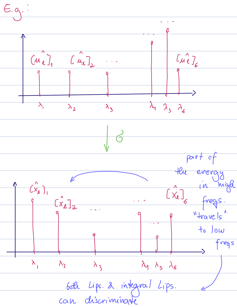
we first get a response $\hat{x}$ from the spectral representation of a convolutional graph filter
after the nonlinearity, some of the energy modes to other areas of the spectrum

Some of the energy in high frequencies "travels" to low frequencies. Both lipschitz graph filters and integral Lipschitz filters can discriminate at these low frequencies.

If any of our task depends on high-frequency data, then this scattering can help us perform well by moving some of the high-frequency information into the lower frequencies, where we have both stability and discriminability

Takeaway

GNNs can perform better than their constituent graph filters. That is, they are more stable for the same level of discriminability, and more discriminative for the same level of stability than a direct composition of the same filters.

This is because the nonlinear activation function "scatters" the signal across the spectrum, moving some high frequency information to lower frequencies and vice versa. Since both lipschitz graph filters and integral Lipschitz filters can discriminate at low frequencies, the mixing from the nonlinearity helps the GNN account for a wider range of the information.

see GNNs perform better than their constituent filters