2025-03-05 graphs lecture 12

[[lecture-data]]

Summary

Last Time

expressivity with respect to the WL test

Today

stability of graph convolution to graph perturbations
discriminability of a graph filter

1. Graph Signals and Graph Signal Processing

Pytorch Things

First: how dataloaders work

Sampling-based GNN training

(1) divide $V$ random batches $V_{b_{1}}, V_{b_{2}}, \dots$

number of batches depends on batch size, a hyperparameter you set
(2) for $i = 1, \dots$ n batches do

for $j \in B_{i}$ (each element in batch)
for $ℓ = 1 \dots L$ (forward pass)

(x_{ℓ})_{j} = σ (\sum_{k = 0}^{K - 1} \sum_{p \in N (j)} [S]_{j p} (x_{ℓ - 1})_{p} H_{k ℓ})

note

only embeddings of $j \in V_{B_{i}}$ are updated (not all of them)

H_{k ℓ}^{(i)} = H_{k ℓ}^{(i - 1)} - η \sum_{j \in V_{B_{i}}, j \in J} \nabla ℓ (y_{j}, (x_{i})_{j})

Where $J \subseteq V$ is the training set. If $J \subset V$ , then the task is semi-supervised and we create a mask over our nodes during training (see Lecture 6 for defining/creating mask)

$j \in V_{B_{i}}$
Loss and weights updates are only computed for the nodes in the batch

Last time intro to PyTorch - see Lecture 11 colab notebook

torch_geometric vs hand-coding: representing graphs as edge lists
convolutions more like sparse matrix multiplications
many benchmarks available including Cora, paper citation network dataset
NeighborLoader is a dataloader for graph nodes
- requires training mask, typically included in canonical datasets

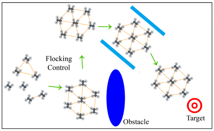
Stability of GNNs to graph perturbations

GNN outputs should be stable. Graphs might have small perturbations, but the outputs should vary as little as possible.

Example

offline controller should still perform well in online trajectories

Example

Recall that permutation equivariance functions as implicit data augmentation, ie, there are symmetries/structures automatically encoded into the data that we can utilize to have better models.

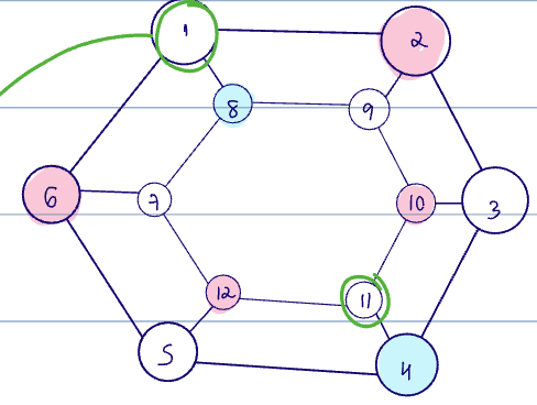
If we observe Node 1's label $y_{1}$ at training time, but not Node 11's, the GNN still learns to output ${\tilde{y}}_{11}$ . The GNN learns the same output for Node 11 as Node 1. Why? The network learns an automorphism of the graph.

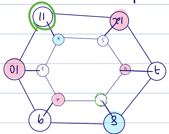
20250310-2025-03-05-graph-1.png|200 maps to 20250310-2025-03-05-graph-2.png|200

In the example above, the automorphism is

P_{y} = H (P S P^{T}) P x = H S x = y

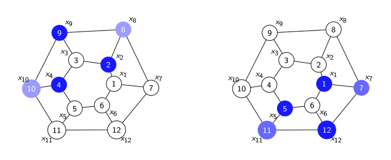
And this means that we don't need to know $y_{11}$ during training time, we only need $y_{1}$ !

graph automorphism

Let $G = (V, E)$ be a graph. A graph automorphism is a graph homomorphism from $G$ to $G$ . That is, a map $γ : G \to G$ such that

(i, j) \in E ⟹ (γ (i), γ (j)) \in E

If there exists an automorphism for $G$ , then there exists a corresponding permutation matrix $P$ such that $V = P V$ .

Note

In a learning task (in a GNN), this means that the shift operator $S = P S P^{T}$ and node features $x = P x$ for the permutation matrix $P$ .

see graph automorphism

We typically want our GNNs to be invariant to automorphisms

Example

In practice, most graphs don't have true automorphisms/symmetries, but quasi-symmetries.

Stability to perturbations ensures "data augmentation behavior" or permutation equivariance under not-quite-symmetries.

operator distance modulo permutations

The operator distance modulo permutations for an operator $ψ : x \mapsto y$ is given by

\begin{aligned} | | ψ - ψ^{'} | |_{p} & = min_{P \in P} max_{x : | | x | | = 1} | | P^{T} ψ (x) - ψ^{'} (P^{T} x) | | \\ = sup_{x : | | x | | = 1} | | P^{T} ψ (x) - ψ^{'} (P^{T} x) | | \end{aligned}

This can be defined for any norm on the LHS, but typically is the operator norm induced by the 2 norm.

Note

For graphs, we can consider $ψ$ to be some graph and $x$ the nodes. This looks for the permutation that makes these graphs closest to one another, then computes a distance.

see operator distance modulo permutations

When $| | S - S^{'} | |_{p} \leq ϵ$ , then we have a quasi-symmetry. (see quasi-symmetry)

Stable Graph Filter

Let $S$ be a graph shift operator and $S^{'} = f_{ϵ} (S)$ some perturbation for some $ϵ > 0$ . Let $H$ be a graph filter. We say $H$ is stable to the perturbation $f$ if

| | S - S^{'} | |_{p} \to 0 as ϵ \to 0

see stable graph filter

graph filters are equivariant to permutations

Recall the definition for a convolutional graph filter:

Linear Shift-Invariant /Convolutional Graph Filters

We define our convolutional graph filter (or linear shift-invariant) as follows. Let $S$ be a graph shift operator and $x$ some graph signal. Then a filter $H$ has
$y = H (S) x = \sum_{k = 0}^{K - 1} h_{k} S^{k} x, h_{0}, h_{1}, \dots, h_{K - 1} \in R$
Note that means $H (S)$ is a $(K - 1)$ th degree polynomial of $S$ with (filter) coefficients $h_{i}$

invariant to permutations

Let $S$ be a graph shift operator. A graph filter $H (S)$ is permutation invariant if $S$ is permutation invariant.

If $S$ is permutation invariant, then since $H$ is also permutation invariant, we have

| | S - S^{'} | |_{p} = 0 ⟹ | | H (S) - H (S^{'}) | |_{p} = 0

For GNNs, we have equivalently $| | S - S^{'} | |_{p} = 0 ⟹ | | Φ (S) - Φ (S^{'}) | |_{p} = 0$ since this is a composed graph convolution

see filter permutation invariance

graph filter stability definitions

lipschitz stable / continuous

A function $f : x \to y$ is $c -$ Lipschtiz stable if

| | f (x) - f (x^{'}) | | \leq c | | x - x^{'} | | \forall x, x^{'}

or if $| | f^{'} (x) | | \leq c \forall x$

(see Lipschitz continuous)

The convolutional graph filter $y = \sum_{k = 0}^{K - 1} h_{k} S^{k} x$ is linear in both $h_{k}$ and $x$ .

(1) if $x^{'} = x + ϵ$ , then $| | y - y^{'} | | \leq (K . max_{k} h_{k} λ_{i}^{+ +})$
(2) if $h_{k}^{'} = h_{k} + ϵ$ , then $| | y - y^{'} | | \leq (λ_{1}^{k} \cdot | | x | |) ϵ$

Because continuous linear functions are lipschitz continuous, graph convolutions are naturally lipschitz and stable to perturbations on both $x$ and $h_{k}$ .

Takeaway

graph convolutions are Lipschitz stable to perturbations in $x$ and $h_{k}$ .

This is because the convolutional graph filter $y = \sum_{k = 0}^{K - 1} h_{k} S^{k} x$ is linear in both $h_{k}$ and $x$ , and continuous linear functions are lipschitz continuous.

(see graph convolutions are stable to perturbations in the data and coefficients)

However, graph convolution is nonlinear in $S$ ... so it is more challenging to determine stability...

Suppose we have a graph shift operator $S$ and some perturbed version $S^{'}$ . To have stability, we want $| | Φ (S) - Φ (S^{'}) | |_{p} \leq c ϵ$ , ie we want this to be Lipschitz for a small constant $c$ .

Recall the spectral representation of a convolutional graph filter:

Spectral Representation of a Convolutional Graph Filter

in the spectral/frequency domain, we have
$\hat{y} = \sum_{k = 0}^{K - 1} h_{k} Λ^{k} \hat{x}$
this representation is completely defined by the polynomial $h (λ) = \sum_{k = 0}^{K - 1} h_{k} λ^{k}$

lipschitz filter

Let $h (λ)$ be the spectral representation of a convolutional graph filter. $h (λ)$ is lipschitz on interval $T \subset R$ means there exists some $c \in R$ such that

| h (λ) - h (λ^{'}) | \leq c | λ - λ^{'} | \forall λ, λ^{'} \in T

This uses the idea that once the filter is fixed, we can think of the representation as sampling along a "spectrum polynomial". Typically, $T = [λ_{min}, λ_{max}]$

see lipschitz graph filter

Example

Note

$c$ can be as large or small as you want. A larger $c$ means the filter is more discriminative, ie better able to tell the difference between different eigenvalues.

Discriminability

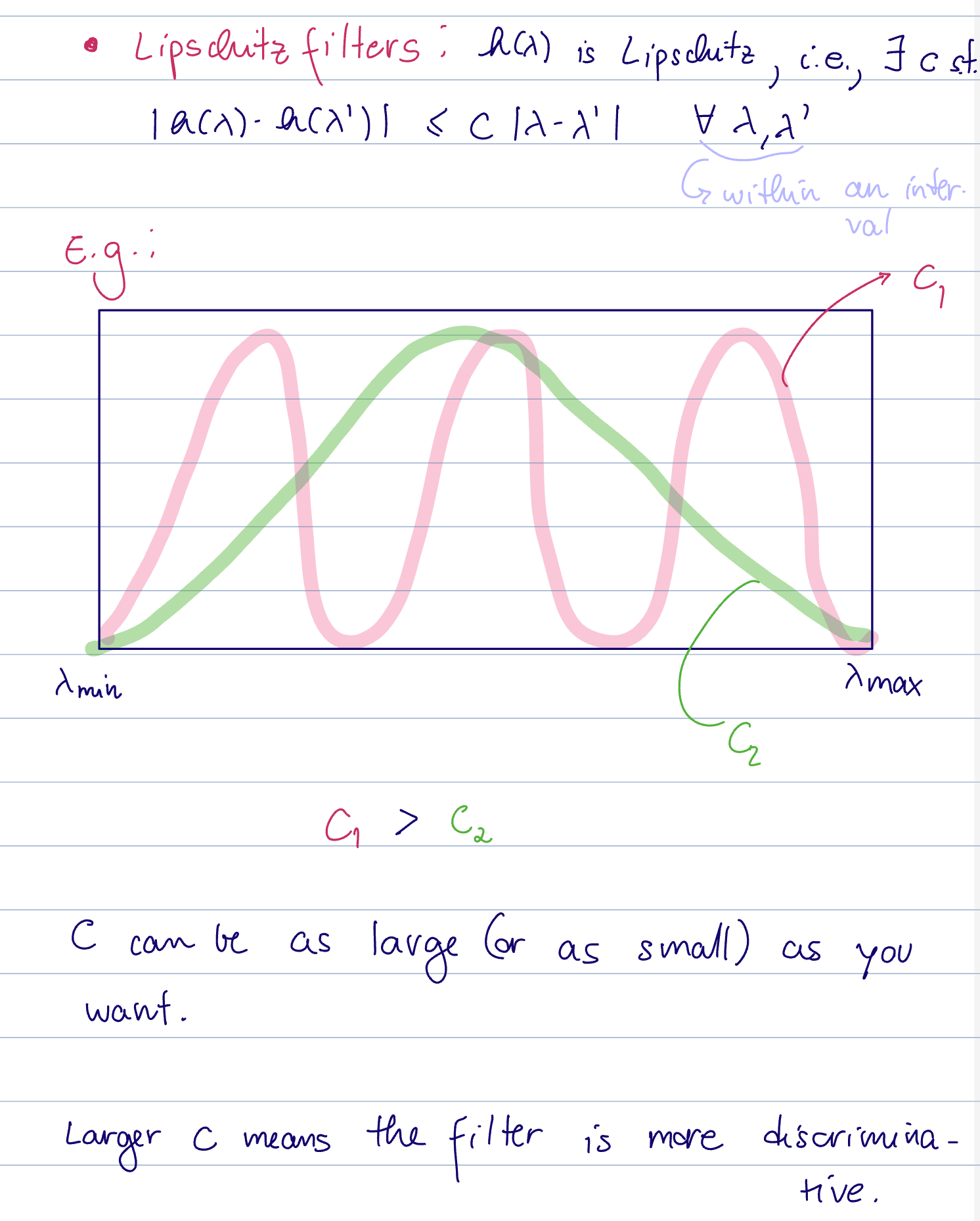
The discriminability of a graph filter describes the ability of the filter to tell the difference between different eigenvalues of the shift operator spectrum.

Recall that we can think of the spectrum as a polynomial in the eigenvalues of the shift operator.

The discriminability thus corresponds with $∣∣ h (λ) - h (λ + ϵ) ∣∣$ , or the change in spectral response for a small change in eigenvalue.

see discriminability of a graph filter

Stability-Discriminability tradeoff for Lipschitz filters

Note that the discriminability is the same at all frequencies. This means there is a tradeoff on benefits between having a large vs a small Lipschitz constant.

with a small $c$ , there is better stability for small perturbations on the eigenvalues
However, if there are large perturbations on the graph, it is good to be more discriminating to notice these changes.

Example Illustration

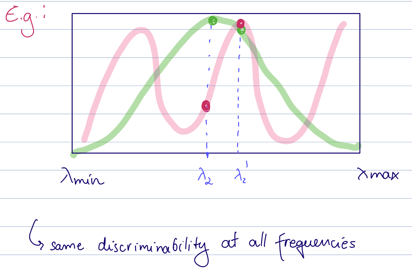
Here, green has a smaller $c$ and pink has a larger $c$ .

$λ_{2}^{'}$ is a perturbation on the second eigenvalue $λ_{2}$ .

The green filter is stable and gives a response that is very close to at both $λ_{2}$ and $λ_{2}^{'}$
whereas the pink filter has a larger difference at the two sampled locations, but has better discriminability

Having a larger Lipschitz constant results in better discrimination between the responses, but less stability.

see stability-discriminability tradeoff for Lipschitz filters

A relaxed version of a lipschitz graph filter is an integral Lipschitz filter.

integral lipschitz filter

Let $h (λ)$ be the spectral representation of a convolutional graph filter. $h (λ)$ is integral lipschitz on interval $T \subset R$ means there exists some $c \in R$ such that

| h (λ) - h (λ^{'}) | \leq \frac{C | λ^{'} - λ |}{\frac{1}{2} | λ + λ^{'} |} \forall λ, λ^{'}

ie, $h (λ)$ is lipschitz with a constant inversely proportional to the interval's midpoint

Letting $λ^{'} \to λ$ , we get $λ h^{'} (λ) \leq c$ and $h^{'} (x) \leq \frac{c}{λ} \to 0$ as $λ \to \infty$

see integral Lipschitz filter

We consider 3 perturbation types (first for graph convolutions, then for GNNs)

operator dilation

$S^{'} = (1 + ϵ) S$ $⟹ | | S - S^{'} | | = ϵ | | S | |$

We can interpret this as the edges being scaled by $(1 + ϵ)$ .

see operator dilation

notes

[p] This is a reasonable perturbation model because the edges change in proportion to their values.
At the same time, it is unrealistic because the proportion is the same for all edges ✅ 2025-03-07
[c] Cannot model edge additions or deletions

Theorem

Let $S^{'} = (1 + ϵ) S$ be a dilation, and consider graph convolution $H (S)$ . If $H (S)$ is a integral Lipschitz filter with constant $c$ , then

| | H (S) - H (S^{'}) | | \leq c ϵ + O (ϵ^{2})

That is, integral Lipschitz filters are stable to dilations.