2025-03-03 graphs lecture 11

[[lecture-data]]

Summary

Last Time

the WL test is at least as powerful as a GNN for detecting graph non-isomorphism

1. Graph Signals and Graph Signal Processing

Recall from last time that injective GNNs are as powerful as the WL test:

Theorem

Let $G_{1}$ and $G_{2}$ be two graphs that the Weisfeiler-Leman Graph Isomorphism Test determines are non-isomorphic. A GNN $Φ$ maps $G_{1}$ and $G_{2}$ to $Φ (G_{1}) \neq Φ (G_{2})$ if the following hold:

$Φ$ aggregates and updates as
$(x_{ℓ})_{v} = ϕ ((x_{ℓ - 1})_{v}, φ ({(x_{ℓ - 1})_{u} : u \in N (v)}))$
Where $ϕ, φ$ are injective.
The readout function is (permutation invariant) and injective.

Graph isomorphism network

A graph isomorphism network (GIN) layer is defined as

(x_{ℓ})_{v} = σ (W_{ℓ} ((1 + ε_{ℓ}) (x_{ℓ - 1})_{v} + \sum_{u \in N (v)} (x_{ℓ - 1})_{u}))

We can write this layer in terms of concatenate function $φ$ :

φ ({(x_{ℓ - 1})_{u} : u \in N (v)}) = \sum_{u \in N (v)} (x_{ℓ - 1})_{u}

And aggregate function $ϕ$

ϕ ((x_{ℓ - 1})_{v}, φ (\cdot)) = W_{ℓ} ((1 + ε_{ℓ}) (x_{ℓ - 1})_{v} + φ (\cdot))

The motivation for this architecture comes from the fact that injective GNNs are as powerful as the WL test, which holds in this case as long as $ϕ, φ$ as defined above are injective.

see Graph Isomorphism Network

Here,

notes

$ϕ_{ℓ} \circ \sum φ_{ℓ - 1}$ is a perceptron or MLP over the neighborhood multiset

Hornik 1989 says an MLP can model any injective function - this is due to the universal approximation theorem
Injective $ϕ_{ℓ} \circ \sum_{X} ϕ_{ℓ - 1}$ exist for multiset $X$ (proven in paper where GINs are introduced)

Can we map an injective function from multisets to embeddings using composition?

Yes, using one-hot encoding of multisets
The function/parameterization is such that it is possible to learn
Original graph isomorphism paper added to the Canvas

Example

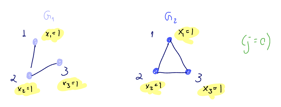
Can a GIN tell them apart? We assume $W_{0} = 1, ε_{0} = 0$ . At the first layer, we take the sum of each node's neighbors' embedding and add it to the node's embedding.

$j = 1$
$G_{1}$

$x_{1} = 1 + 1 = 2$
$x_{2} = 1 + 1 + 1 = 3$
$x_{3} = 2$
output is ${2, 3, 2}$
$G_{2}$
$x_{1} = x_{2} = x_{3} = 3$
output is ${3, 3, 3}$

As long as we have an injective function from multisets to embeddings, we are OK since we will be able to distinguish between these. To confirm we have this, we look at the graph level readout.

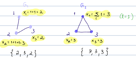
In the GIN paper, the readout is defined in terms of a readout at each layer.

Example

For the example above,

X_{G} = CONCAT (readout ({(x_{ℓ})_{v} : v \in V}) | ℓ = 1, 2, \dots, L)

And so

$G_{1} : [3 | 7]$
$G_{2} : [3 | 9]$

Note

The concatenation is not needed, but the authors claim better generalization
- the order of the concatenation doesn't matter as long as it is consistent for each graph
with the sum as the readout, the GIN generalizes the WL test

Takeaway

thus, a GIN is a maximally powerful GNN in graph-level tasksfor anonymous inputs (ie $\vec{x} = 1$ )

see GINs are maximally powerful for anonymous input graphs

Is being as powerful as the WL test enough?

Example

Can WL test distinguish between the two graphs below?

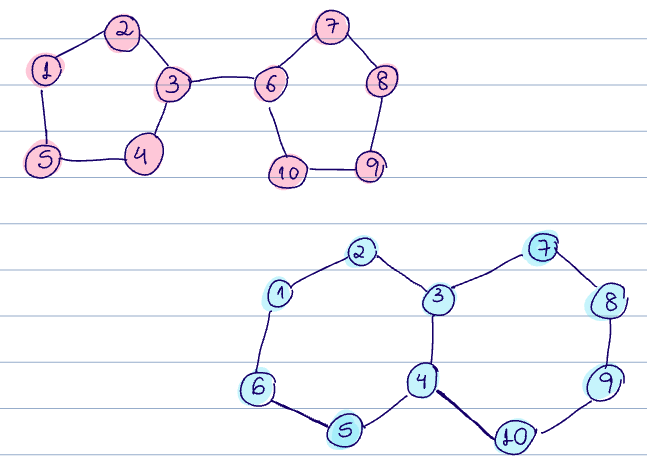
The output of the color refinement algorithm for Graph 1 gives:

1, 2, 3, 4, 5, 7, 8, 9, 10 have color 1
3, 6 have color 2

And for Graph 2:

1,2,5,6, 7,8,9,10 have color 1
3,4 have color 2

So in this case, the multisets of the colors are the same between G1 and G2, and we cannot distinguish between them.

So, NO! Thus, the computational graphs are the same, despite these being different graphs.

Exercise

Check

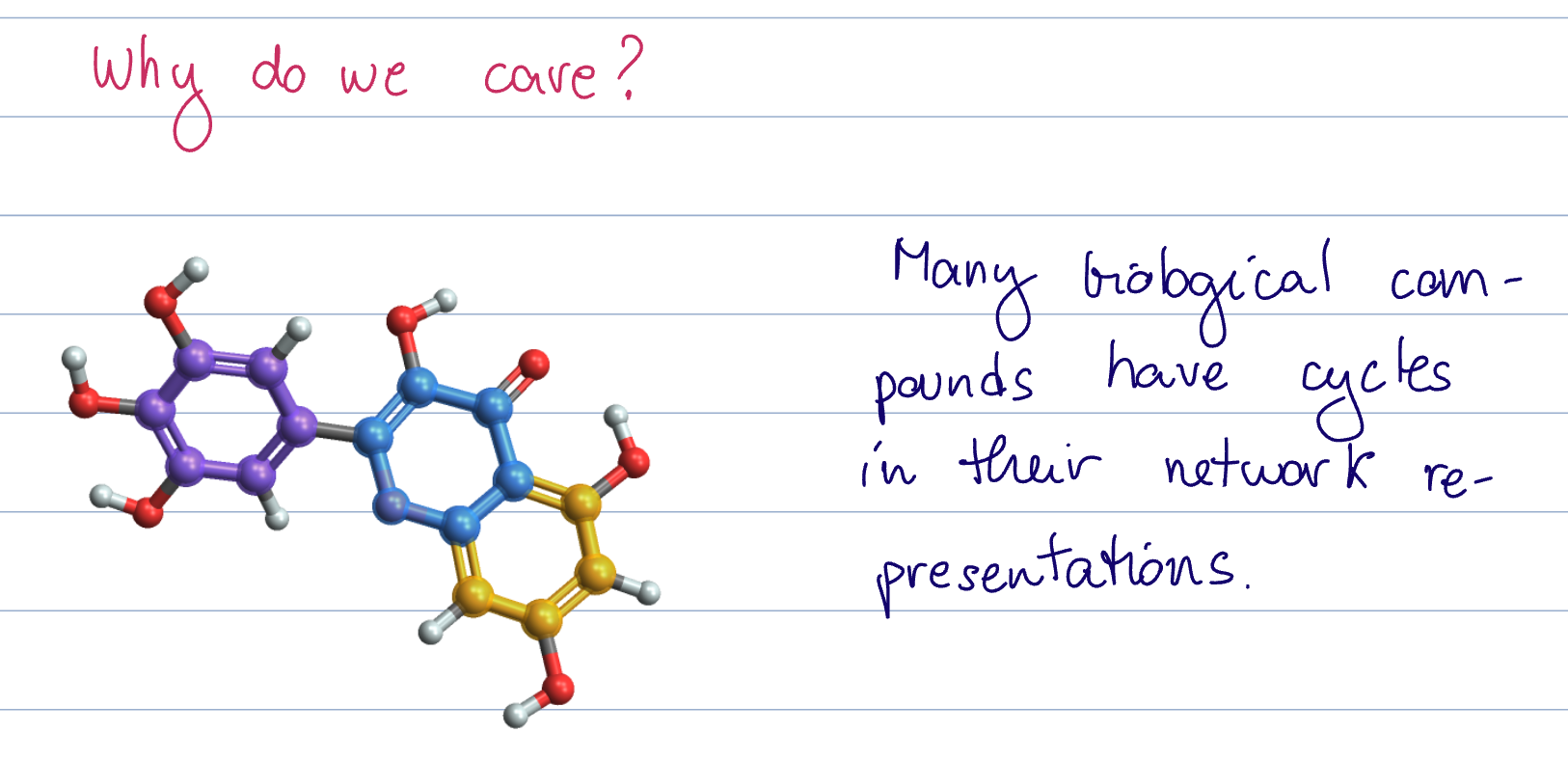
Instead, we could count the number of cycles to see if these graphs are different.

2 cycles in graph1
3 cycles in graph2

$⟹$ If we had a GNN that could count cycles, we could discriminate between these graphs.

But GNNs are less powerful than the WL test, so GNNs could not discriminate between these graphs. And this implies that they cannot count cycles.

There is another way to count cycles: densities of cycle homomorphisms

Graph Homomorphism

Let $G = (V, E)$ and $F = (V^{'}, E^{'})$ . A graph homomorphism from $F$ to $G$ is a map $γ : F \to G$ such that

(i, j) \in E^{'} ⟹ (γ (i), γ (j)) \in E^{'}

ie, homomorphisms are adjacency-preserving maps (of $F$ )

see graph homomorphism

Exercise

How is a homomorphism not the same as a graph isomorphism?

Answer

Recall the definition of the isomorphism

Graph Isomorphism

Let $G$ and $G^{'}$ be two graphs. A graph isomorphism between $G$ and $G^{'}$ is a bijection $M : V (G) \to V (G^{'})$ such that for all $i, j \in V (G)$
$(i, j) \in E (G) ⟺ (M (i), M (j)) \in E (G^{'})$

The isomorphism requires that both graphs share all edges. The homomorphism requires that the second graph, $G$ , is a subgraph of the first, $F$ .

Example
+++see notes

A valid homomorphism is

We will denote the total number of homomorphisms from $F$ to $G$ as $hom (F, G)$ .

homomorphism density

Let $G = (V, E)$ and $F = (V^{'}, E^{'})$ be graphs. The homomorphism density from $F$ to $G$ , denoted $t (F, G)$ is given as

t (F, G) = \frac{hom (F, G)}{| V |^{| V^{'} |}}

Where $hom (F, G)$ is the the total number of homomorphisms from $F$ to $G$

see homomorphism density

claim

Let $C_{k}$ be the $k$ -cycle. Let $G$ be a graph with adjacency matrix eigenvalues $λ_{1}, λ_{2}, \dots, λ_{n}$

For $k \geq 4$ , we have

t (C_{k}, G) = \frac{(\sum_{i} λ_{i}^{k})}{n^{k}}

Where $t (\cdot)$ is the homomorphism density

Proof

Note that

hom (C_{k}, G) = \sum_{i, j, k, ℓ, \dots} (A_{i j} A_{j k}) A_{k ℓ} A_{ℓ m} \dots A_{ζ i}

= \sum_{i, k, ℓ} \sum_{j} (A_{i j} A_{j k}) A_{k ℓ} A_{ℓ m} \dots A_{ζ i}

= \sum_{i, k, ℓ} [A^{2}]_{i k} A_{k l} A_{ℓ m} \dots A_{ζ i}

= ⋮

= \sum_{i} [A^{k}]_{i i} = Tr (A^{k}) = \sum_{i} λ^{k}

Thus $t (c_{k}, G) = \frac{\sum_{i} λ_{i}^{k}}{n^{k}}$

Note

This implies that cycles can be counted using a convolutional GNN with white input (see Lecture 9) with graph shift operator $S = \frac{A}{n}$ .

see cycle homomorphism density is given by the trace of the adjacency matrix

we can set $h_{k}$ to be 1 for the nodes we want in the cycle
+++note/distill how to get the cycle density using this type of algorithm

To be able to count these cycles, we need the input to be white. For the GIN, we needed to have the inputs to be anonymous ie each $x_{i} = 1$ .

For this method to work, we need each ${\hat{x}}_{i} = 1$ , ie anonymous in the spectral domain.

This means that white inputs help improve expressivity (as opposed to anonymous inputs $x_{i} = 1 \forall i$ )

The "best of both worlds" can be achieved by merging the two methods: using a GIN with white inputs

Since designing a white inputs requires computing eigendecomposition, we usually relax this condition to random inputs instead, which almost surely satisfy ${\hat{x}}_{i} = 1$ .

Takeaway

For maximum expressivity, we can use a GIN with white, anonymous inputs. That is,

Each $x_{i} = 1$
Each ${\hat{x}}_{i} = 1$

However, designing a white inputs requires computing eigendecomposition which is expensive.

Instead, we usually relax this condition to random inputs, which almost surely satisfy ${\hat{x}}_{i} = 1$ .

see random graphs in a gin are good for graph isomorphism

TBC in HW2

Detour:

properties of GNNs
- permutation equiv
- expressivity
- limitations/advantages of conv archs
Next:
- stability to perturbations

Detour:

implementations in PyTorch Geometric

see lecture 11 notebook
torch_geometric

graphs no longer represented as adjacency matrices
something similar to sparse matrix representations

Node features represented as $n \times d$ tensor

to_networkx from torch_geometric.utils
to convert to networkx object to plot :)

In general, going to use benchmark datasets

citation network, classify into communities

see notebook for defining a GNN in pyG - have layers implemented already