2025-02-12 graphs lecture 7

[[lecture-data]]

2025-02-12

Summary

2025-02-10 graphs lecture 6

This Time

information theoretic lower threshold
community detection

1. Graph Signals and Graph Signal Processing

information theoretic threshold

Recall from last time that in the balanced sbm with $C = 2$ , if $p \approx q$ , there is a region around $p = q$ where the detection of communities is impossible from an information theory perspective using the signal to noise ratio.

Example

In our example with $c = 2$ , with $B = {\begin{cases} p if c_{1} = c_{2} \\ q otherwise \end{cases}$ , then
$S N R = \frac{(p - q)^{2}}{2 (p + q)}$

numerator is the signal: degree discrepancy in nonequal subgraphs
denominator is noise: the average degree for all nodes in the graph

Theorem

Suppose we have a stochastic block model problem where the adjacency matrix $A \sim P, P = Y B Y^{T}$ , and $B = {\begin{cases} p if c_{1} = c_{2} \\ q otherwise \end{cases}$ .

If the signal to noise ratio $S N R \frac{< 1}{n}$ , then almost exact recovery is impossible.

Even with infinite time and resources, there is no algorithm that can recover the true communities with just the probabilities of adjacency. This gives us the information theoretic threshold

Proof

see proofs in Massoulié (2014) and Mossel (2014). Aside: interesting to see since there are different proof methods from different domains. See also Abbe (survey papers).

Example: Sparse Graphs

$p = \frac{a}{n}, q = \frac{b}{n}$ and $\frac{| E |}{n^{2}} \to 0$ as $n \to \infty$ (the average degree vanishes).
Then
$\begin{aligned} S N R & = \frac{{(\frac{a}{n} - \frac{b}{n})}^{2}}{2 \frac{(a + b)}{n}} \\ = \frac{1}{2 n} \frac{(a - b)^{2}}{(a + b)} \\ S N R_{p, q} < \frac{1}{n} & ⟺ \frac{1}{2 n} \frac{(a - b)^{2}}{a + b} < \frac{1}{n} \\ ⟹ \frac{(a - b)^{2}}{2 (a + b)} & < 1 \end{aligned}$
ie, in sparse graphs, it is not difficult to identify the information theoretic threshhold (we can easily calculate the signal to noise ratio)

Takeaway

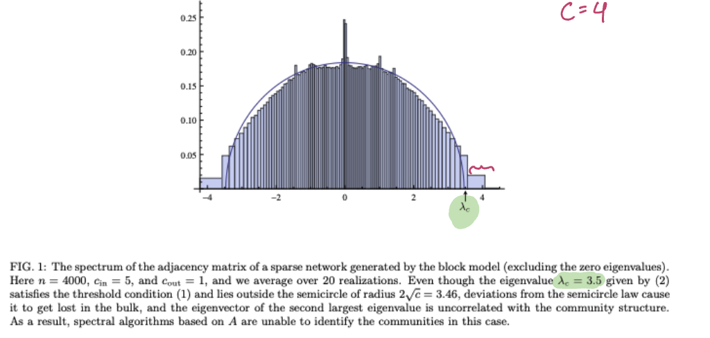
Community detection is difficult when the graph is sparse. Traditional methods may fail even before we hit this threshold!

contextual stochastic block model (C-SBM)

The (binary) contextual stochastic block model (C-SBM) is like an SBM, but includes node features that are drawn from a Gaussian distribution. Here,

The adjacency matrix is given as $A : A_{i j} = A_{j i} \sim Bernoulli (P_{i j})$ where

P \in R^{(n / 2 + n / 2) \times (n / 2 + n / 2)} = [\begin{array}{cccccc} p & \dots & p & q & \dots & q \\ ⋮ & ⋮ & ⋮ \\ p & \dots & p & q & \dots & q \\ q & \dots & q & p & \dots & p \\ ⋮ & ⋮ & ⋮ & ⋮ \\ q & \dots & q & p & \dots & p \end{array}]

$y \in {- 1, 1}^{n}$ (or ${0, 1}$ ) and $B \in R^{2 \times 2}$
And node features $X$ are drawn
$x_{i} \sim \sqrt{\frac{μ}{n}} y_{i} u + \frac{z_{i}}{\sqrt{d}}$ , $u \sim Normal (0, \frac{I_{d}}{d})$ , $z_{i} \sim Normal (0, I_{d})$

X_{i} | Y_{i}, u \sim Normal (\pm \sqrt{\frac{μ}{n}} u, \frac{I_{d}}{d})

(see contextual stochastic block model)

Feature-aware spectral embeddings

Recall that is spectral clustering, which is fully unsupervised. For spectral embedding, we make use of some of the known community assignments.

feature-aware spectral embeddings

Feature-aware spectral embeddings incorporate the availability of node features into our predictions (for example, in a C-SBM) when using spectral embedding.

Let $G$ be a graph with diagonalizable adjacency matrix $A$ and node features $X \in R^{n \times d}$ . Suppose we have $C$ communities that we want to assign to the nodes.

Diagonalize $X X^{T} \in R^{n \times n}$ as $\tilde{V} Λ {\tilde{V}}^{T}$
Pick the top $κ$ eigenvectors to create ${\tilde{V}}_{(κ)} \in R^{n \times κ}$
Define $V_{c + κ} = [V_{c} | {\tilde{V}}_{(κ)}]$ where $V_{c}$ are the top $C$ eigenvectors of $A$ .

(see feature-aware spectral embeddings)

Before, we had

Spectral Embedding Problem

$min_{f} \sum_{i \in T} 1 (f (A)_{i} = y_{i}), f \in {f (A) = σ (V_{c} W), W \in R^{C \times C}}$

Now, our hypothesis class is instead:

Feature-Aware Spectral Embedding Hypothesis Class

f (A, x) = σ (V_{c + κ} W), W \in R^{(c + κ) + (c + κ)}

Note

In the presence of node features, the information theoretic threshold for community detection becomes (with $p = \frac{a}{n}, q = \frac{b}{n}$ )

S N R (A) + S N R (x) = \frac{(a - b)^{2}}{2 (a + b)} + \frac{μ^{2} d}{n} > 1

Takeaway

the community detection is possible in an information theoretic sense when $p \approx q$ as long as the means of the communities are sufficiently separated (high $μ$ and/or high $d$ ).

Computational thresholds for spectral clustering (non-rigorous)

maybe there exists an algorithm that can find these communities, but can we do so in polynomial time? Can we do even better?

Example

spectral redemption - Krzkala et al 2013. Computational threshold using adjacency matrix

Takeaway

Even by doing spectral embedding or feature-aware spectral embeddings, since we have to fix $c$ (which is often unknown) and $κ$ (the number of eigenvectors we use) our spectral algorithms might fail.

In practice, spectral algorithms fail above the information theoretic threshold (sometimes, significantly above that threshold!)

(see sometimes spectral algorithms fail)

Question

Can GNNs help?

Answer

Let's go back to Lecture 3. We saw that the expressivity of graph convolutions can find regression solutions in many cases

Recall the conditions for finding a convolutional graph filter:

Theorem

Let $S$ be a shift operator with eigenvalues $λ_{1}, λ_{2}, \dots, λ_{n}$ , and $x$ a graph signal. Let $\hat{x}$ be the GFT.

Suppose

${\hat{x}}_{i} \neq 0 \forall i$
$λ_{i} \neq λ_{j} \forall i \neq j$

Then there exist $K \leq n$ coefficients $h_{0}, \dots, h_{K - 1}$ such that $y = H (S) x$ , and $H$ is a graph convolution

In the example above, having access to $C^{'} > C$ eigenvectors might have helped. But not only do we need to fix $C$ when unknown, we also have to pick a large enough $C$ so that we don't miss informative eigenvalues "lost in the bulk" like in the paper.

This motivates using GNNs for semi-supervised community detection on graphs

Takeaway

We can use GNNs to solve the semi-supervised community detection node-level task on graphs.

Let $G$ be a graph with diagonalizable adjacency matrix $A$ and node features $X \in R^{n \times d}$ . Suppose we have $C$ communities that we want to assign to the nodes.

As long as $X$ satisfies the conditions for finding a convolutional graph filter, namely that

${\hat{x}}_{i} \neq 0 \forall i$ and
$λ_{i} \neq λ_{j}$ for all $i \neq j$

then there exists a graph convolution (or a 1-layer linear GNN) that approximates $y$ . The optimization problem then is the same as before:

Community Detection Optimization Problem

$min_{f} \sum_{i \in J} ℓ (f (A, X)_{i}, y_{i})$

where $ℓ (\cdot)$ is a surrogate of the 0-1 loss, each $y_{i}$ is the one-hot community vector of node $i$ , and $f$ is some parametric function of $A$ and $X$

And we can choose our hypothesis class so that $f (A, X) = Φ_{H} (A, X)$ , a GNN with learnable parameters $H$ (this is the form of the function we defined in lecture 5)

(see we can use GNNs to solve feature-aware semi-supervised learning problems)

Housekeeping

Homework due 2 weeks from today (first week of)

A note on sparse matrix-vector multiplications

$S x$ , $S^{k - 1} x = S^{k - 2} S x$

the usual matmul operation in PyTorch requires $O (n^{2})$ to compute $S x : (S x)_{i} = \sum_{j = 1}^{n} A_{i j} x_{j}$ for $1 \leq i \leq n$

Example

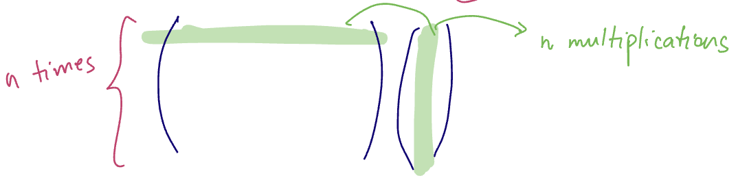
Illustration to see the $n^{2}$ operations required

Typically the graph shift operator $S$ (ie, adjacency matrix $A$ , graph laplacian $L$ , etc) are sparse $n \times n$ matrices, ie $\frac{| E |}{n^{2}} ≪ 1$

in this case, $| E |$ nonzero entries can achieve $O (| E |)$ complexity. But, to achieve it you need to use the sparse tensor representation of $S$

How sparse `matmuls` work

Suppose we have a sparse adjacency matrix

A = [\begin{matrix} 12 & 0 & 26 & 0 \\ 0 & 0 & 19 & 14 \\ 26 & 19 & 0 & 0 \\ 0 & 14 & 0 & 7 \end{matrix}]

There are two main options to store this more efficiently.

Coordinate (COO)rdinate Representation

$A$ can become a set of $| E |$ tuples of the form $(row index, column index, value)$ . So this matrix becomes the ordered set of these tuples, sorted by row and then column index.

This can be better from a memory perspective, but can still be quite large if we have a few nodes with high degree. A nice solution to this is to use compressed sparse row representation instead.
(see coordinate representation)

Example

$A = [\begin{matrix} 12 & 0 & 26 & 0 \\ 0 & 0 & 19 & 14 \\ 26 & 19 & 0 & 0 \\ 0 & 14 & 0 & 7 \end{matrix}]$

can become
$(0, 0, 12), (0, 2, 26), (1, 2, 19), (1, 3, 14), (2, 0, 26), (2, 1, 19), (3, 1, 14), (3, 3, 7)$

Another method to compress a sparse matrix's information is through compressed sparse row (CSR) representation - this is most popular.

Compressed Sparse Row (CSR) representation

Suppose $A \in R^{n \times m}$ is a sparse matrix. We can represent it as a set of 3 tensors/"lists" called compressed sparse row representation (CSR). We get this representation by realizing that we can encode the row index in the COO representation a bit more efficiently.

Instead of writing out the row index for each element, we can collect the column indices for each row, put each of these collections together, and then have a pointer tell us where to start reading.

If $A$ has $z$ non-zero entries, then

the column tensor contains $z$ entries. Each entry contains the column index for one of the non-zero elements, sorted by ascending row index.
row or pointer tensor contains $n + 1$ entries
- the first $n$ entries contain the starting index for where the row's elements start in the column tensor
- the last entry is $z$
value tensor contains $z$ entries and contains the non-zero elements sorted by row then column index.

(see compressed sparse row representation)

Example

$A = [\begin{matrix} 12 & 0 & 26 & 0 \\ 0 & 0 & 19 & 14 \\ 26 & 19 & 0 & 0 \\ 0 & 14 & 0 & 7 \end{matrix}]$

Pointer = [0 2 4 6]

\begin{array}{ccccc} index & 0 & 1 & 2 & 3 \\ read start & 0 & 2 & 4 & 6 \end{array}

Column = [0 2 2 3 0 1 1 3]

\begin{array}{ccccccccc} index & 0 & 1 & 2 & 3 & 4 & 5 & 6 & 7 \\ col indx & 0 & 2 & 2 & 3 & 0 & 1 & 1 & 3 \end{array}

Value = [12 16 19 14 26 19 14 7]

\begin{array}{ccccccccc} index & 0 & 1 & 2 & 3 & 4 & 5 & 6 & 7 \\ value & 12 & 26 & 19 & 14 & 26 & 19 & 14 & 7 \end{array}

Matrix multiplication can then become much more efficient computationally. Using sparse matrix multiplication we get

total operations = \sum_{i = 1}^{n} | N_{i} | = \sum_{i = 1}^{n} d_{i} = 1^{T} A 1 = | E |

in PyTorch, to transform to a sparse tensor:

S.to_sparse() for COO
S.to_sparse_csr() for CSR

matrix-vector multiplication is as before: S @ x or torch.mv(S,x) for both representations and this will give a faster multiplication.

1. Graph Signals and Graph Signal Processing

information theoretic threshold

contextual stochastic block model (C-SBM)

Feature-aware spectral embeddings

Computational thresholds for spectral clustering (non-rigorous)

A note on sparse matrix-vector multiplications

How sparse matmuls work

How sparse `matmuls` work