2025-02-03 graphs lecture 4

Data

subject:: Data Science Methods for Large Scale Graphs

Clean: INPUT[toggle(offValue(0), onValue(1)):clean] Linked: INPUT[toggle(offValue(0), onValue(1)):linked] Publish: INPUT[toggle(offValue(0), onValue(1)):dg-publish]
Maturity: INPUT[inlineSelect(option(seed), option(sprout), option(sapling), option(tree), option(snag), defaultValue(sprout)):maturity]

2025-02-03

Summary

Last time

Today

Filter design
Spectral filters
filter learning
- statistical learning and ERM
- Types of learning problems on graphs

1. Graph Signals and Graph Signal Processing

Example

Suppose we want to design a lowpass filter for some graph signal.

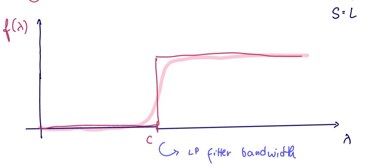
(What does this mean? Consider radio stations: these have carrier waves, which are at higher frequencies than the information to be broadcast. We would need a way to get rid of the carrier frequency to get the desired signal)

Suppose we want to implement this using graph convolutions. Recall that we can represent any analytic function with convolutional graph filters.

Question

Is this function analytic?

Answer

No, but we can often find good analytic approximations of non-analytic functions. For heaviside functions such as the lowpass filter, a good approximation is the logistic function

\tilde{f} (λ) = \frac{1}{1 + e^{- α (λ - c)}}

Where $α$ is a steepness constant

Note

We can approximate heaviside functions using the logistic function as a proxy for our target function

Proof

Logistic functions are analytic, and recall that we can represent any analytic function with convolutional graph filters.

As an illustration, we want to find coefficients $h_{k}$ such that $\sum_{k = 0}^{K - 1} h_{k} λ^{k} = \tilde{f} (λ)$ ,

\tilde{f} (λ) = \frac{1}{1 + e^{- α (λ - c)}}

Here,

\begin{aligned} \tilde{f} (0) & = \frac{1}{1 + e^{α c}} \\ {\tilde{f}}^{'} (λ) = \frac{1}{(1 + e^{- α (λ - c)})^{2}} e^{- α (λ - c)} + α ⟹ {\tilde{f}}^{'} (0) & = \frac{α e^{α c}}{(1 + e^{- α c})^{2}} \\ {\tilde{f}}^{″} (λ) = \frac{- α^{2} e^{- α (λ - c)}}{(1 + e^{- α (λ - c)})^{2}} + \frac{2 α e^{- 2 α (λ - c)} + α}{(1 + e^{- α (λ - c)})^{3}} \\ ⟹ {\tilde{f}}^{″} (0) & = \frac{α^{2} e^{α c}}{(1 + e^{- α c})^{2}} (\frac{2 e^{α c}}{(1 + e^{- α c})} - 1) \\ ⋮ \end{aligned}

Then $h_{0} = \tilde{f} (0), h_{1} = {\tilde{f}}^{'} (0), h_{2} = \frac{{\tilde{f}}^{″} (0)}{2}$ etc.

(see approximation of heaviside functions using convolutional graph filters)

So we can do this. That's great! But it can be costly to compute this approximation, especially the higher order derivatives of this function. Is there a better way to design such a filter?

Spectral Graph Filters

Let $S = V Λ V^{*}$ , $\hat{x} = V^{*} x$ for some diagonalizable shift operator $S$ and some graph signal $x$ .

y = \sum_{j = 1}^{n} c_{j} {\hat{x}}_{j} v_{j}

Where $\hat{x}$ is the graph fourier transform of signal $x$ . We design or learn the constants $c_{j}$ .

(see spectral graph filter)

Example

Let $S = L$ with this spectrum:

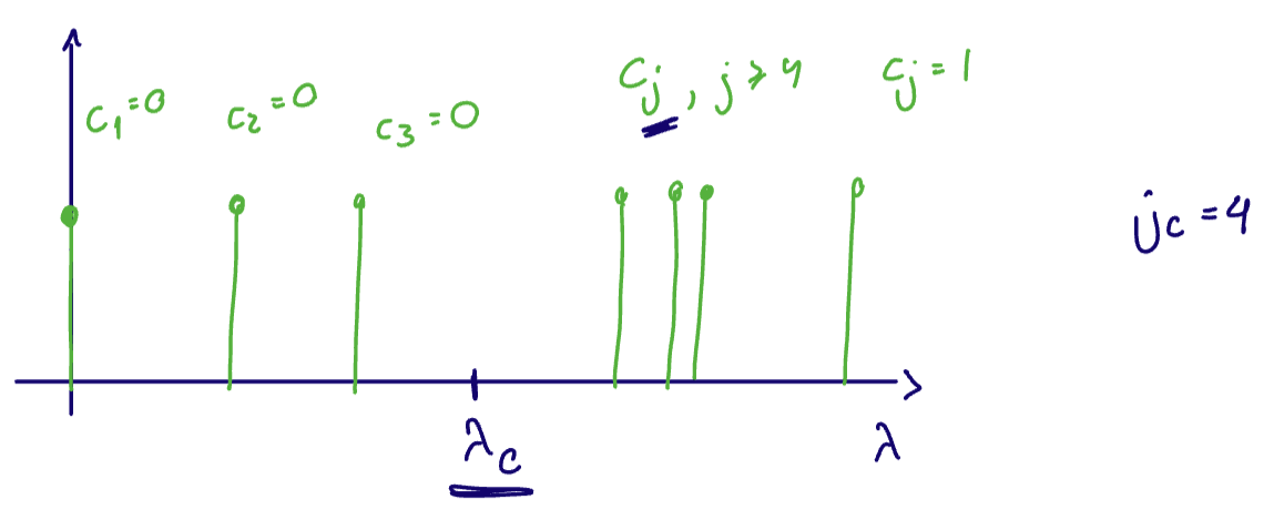
Suppose we want a lowpass filter with bandwith $λ_{c}$ . Then we can simply truncate the spectrum to only allow the frequencies falling below our cutoff (in practice we usually select $j_{c}$ , or the index instead of the actual eigenvalue)

In model applications, we have moved away from system engineering to learning systems from data.

Supervised Statistical Learning

Suppose $x$ and $y$ are related by a statistical model $p (x, y)$ . We are interested in predicting $y$ from $x$ using either $p (y | x)$ or $E (y | x)$ . In practice, we can only estimate these quantities using a model $\tilde{y} = f (x), f \in F$ , where $f$ comes from a function or hypothesis class $F$

How do we pick the best estimator $f$ ? This is the statistical risk minimization problem

Define a loss function $ℓ (y, \hat{y})$ measuring the "cost" of predicting $y = f (x)$ when the output is $y$

Statistical Risk Minimization Problem

Suppose $x, y$ are related by some (known) statistical model $p (x, y)$ , and we want to estimate $p (x, y)$ using a model $\tilde{y} = f (x)$ , where $f$ is a member of our hypothesis class $F$ .

Let $ℓ (y, \hat{y})$ be our loss function. Then the statistical risk minimization problem is to minimize the expected loss over distribution $p (x, y)$ :

f^{*} = \arg min_{f \in F} E_{p (x, y)} {ℓ (y, f (x))}

The optimal estimator $f^{*}$ is the function $f \in F$ with minimal expected cost over all possible functions $f$ .

Note

Typically, we are interested in either

Predicting $y$ from $x$ with the convolutional distribution $y \sim p (y | x)$ .
ex: stochastic outputs: VAEs, diffusion, etc
Predicting $y$ from $x$ with the conditional expectation $y = E (y | x)$
ex: deterministic outputs, classical regime/supervised learning

(see statistical risk minimization problem)

Question

What is the issue with this?

Answer

In practice we only have access to the data. So instead, we can only estimate the risk according to the data

Consider again the statistical risk minimization problem where we wish to estimate $y = f (x)$ from some known distribution $p (x, y)$ . In practice, we typically do not have access to the distribution $p (x, y)$ , we only have access to samples $T = {x^{j}, y^{j}}_{j = 1}^{M}$

Empirical risk minimization problem

Suppose we have samples $T = {x^{j}, y^{j}}_{j = 1}^{M}$ , where $x, y \sim p (x, y)$ and $p (x, y)$ is unknown. Let $ℓ (y, \hat{y})$ be our loss function and $F$ our hypothesis class. Then the solution to the empirical risk minimization problem is

f^{*} = \arg min_{f \in F} \frac{1}{M} \sum_{j} ℓ (y^{j} f (x^{j}))

ie we minimize the empirical mean

Example

Typical loss functions for the ERM are

quadratic / $L^{2}$ loss $ℓ (x, z) = \frac{| | y - z | |^{2}}{2}$ for regression/estimation problems
$0 - 1$ loss $ℓ = I_{(y \neq z)}$ for classification problems
- since we often require differentiation, this is often replaced with a differentiable surrogate like cross entropy loss or logistic loss

Note

The ERM problem might have a closed-form solution (line in linear regression), but in modern ML, it is solved using optimization algorithms such as SGD or ADAM.

Types of Graph Signal Processing Problems

Question

Where do our filters fit into ERM?

Answer

Our hypothesis class are graph convolutional filters

We usually see 3 types of problems

Graph Signal Processing Problem

In a graph signal processing problem (or graph regression or signal regression), the graph $G$ is the data support, and is thus fixed. The data are graph signals $x \in R^{n}$ and we want to predict signals $y \in R^{n}$ . Assuming $x, y \sim p (x, y)$ , we regress signals $y$ on predictor signals $x$ .

Here, the hypothesis class are the graph convolutions $F$ $= {z = \sum_{k = 0}^{K - 1} h_{k} S^{k} x, h_{k} \in R}$

Our minimization problem is then $$\min_{h_{k}} \frac{1}{M}\sum_{j} \ell\left( y^{(j)}, \sum_{k=0}^{K-1}h_{k} S^k x^k \right)$$

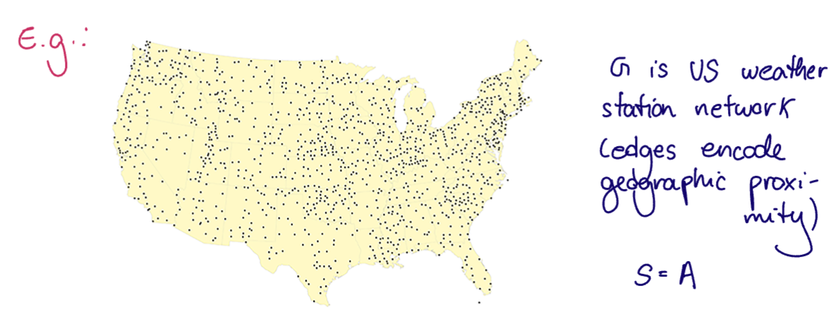
(see graph signal processing problem)

Example

The fixed graph is the US weather station network. Suppose we have our $y$ , the recorded temperatures from February 3 from the last $n$ years, and our $x$ , the recorded temperatures from November 3 from the last $n$ years.

Temperatures on the graph are recorded as time series and
we want to predict the february temperatures from the november temperatures.

Application: temperature forecasting. Predict february 2026 temperatures $(y^{'})$ from the november 2025 temperatures $(x^{'})$ as

y^{'} \approx \sum_{k = 0}^{K - 1} h_{k}^{*} S^{k} x^{'}

Using $L^{2}$ loss, our minimization problem becomes:

min_{h_{k}} \frac{1}{M} \sum_{j} {| | y^{(j)} - \sum_{k = 0}^{K - 1} h_{k} S^{k} x^{k} | |}_{2}^{2}

Graph-Level Problems

In graph-level problems, there are multiple graphs. Each graph $G$ represents a predictor associated with an observation $y \in Y$ . We assume that $G, y \sim p (G, y)$ and want to regress $y$ on $G$ .

Here, our hypothesis class is $F =$ ${f (S) = \sum_{k = 1}^{K - 1} h_{k} S^{k} 1 | h_{k} \in R}$

Note

Since there are no graph signal observations, we use the vector of all ones $1$ as our constant signal!

And our minimization problem is given by $$\min_{h_{k}} \frac{1}{m} \sum_{i=1}^M \ell\left( \sum_{k=0}^{K-1} h_{k} S^k \mathbb{1}, y \right)$$
(see graph-level problem)

Example

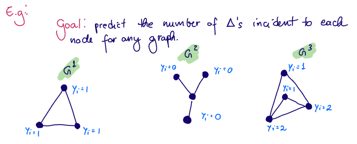
Suppose we want to predict the number of triangles incident to each node for any graph

In this example, since our output is an integer, it mades sense to use the $0 - 1$ loss or a surrogate:

min_{h_{k}} \frac{1}{m} \sum_{i = 1}^{M} ℓ (\sum_{k = 0}^{K - 1} h_{k} S^{k} 1, y)

Application: automate triangle counting

Observation

Both the graph signal processing problem and the graph-level problem are supervised learning (sometimes called transductive learning) problems. ie none of the test inputs are seen at training time.

(see supervised learning)

Node-Level Tasks

Node-Level tasks

Node-level tasks (sometimes called inductive learning or semi-supervised learning) have graph $G$ as the data support (ie, it is fixed). Here, we examine each node as a sample, ie we assume that the signal and observation at node $i$ is $x_{i}, y_{i} \sim p (x, y)$ . ie, each node is treated as a sample.

We assume we only observe $y_{i}$ for a subset of the nodes $J \subset V$ and want to estimate $y_{j}, j \in V ∖ J$

(see node-level task)

Example

Consider the contextual SBM: $G = (V, E)$ undirected and $y \in {- 1, 1}^{n}$ (say $y_{i}$ represents the community of node $i$ ). The edges are random: $P (A_{i j}) = P ((i, j) \in E) = {\begin{cases} \frac{a}{n}, y_{i} = y_{j} \\ \frac{b}{n}, otherwise \end{cases}$ with node features/covariates
$x_{i} = \sqrt{\frac{u}{n}} y_{i} u + z_{i}$ where $u \sim N (0, 1), z \sim N (0, I_{n})$

If $u = 1$ then $x_{i} \sim N (\sqrt{\frac{1}{n}} u, 1)$ and
if $u = 0$ then $x_{i} \sim N (- \sqrt{\frac{1}{n}} u, 1)$

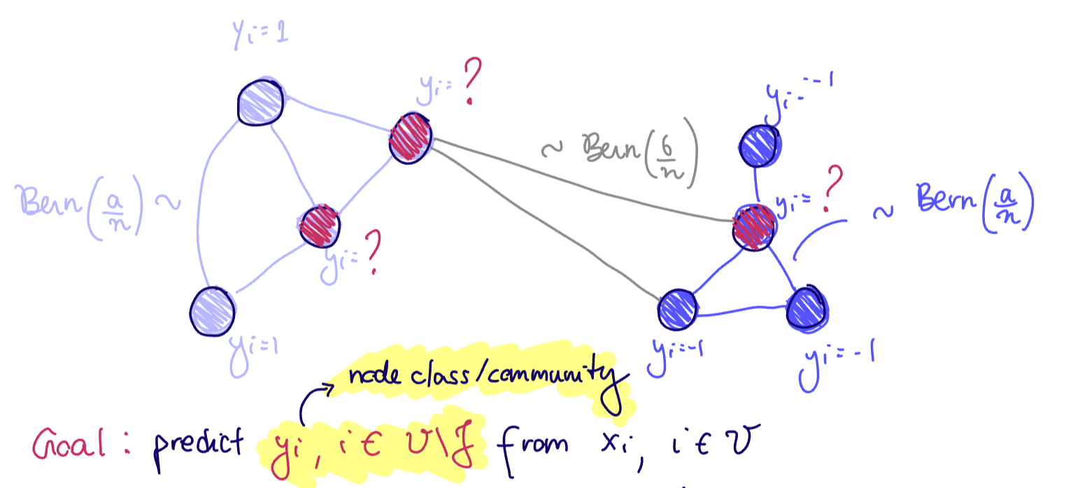
Goal: predict $y_{i}, i \in V ∖ J$ from $x_{i} \in V$
hypothesis class: the graph convolutions $F =$ ${z = \sum_{k = 0}^{K + 1} h_{k} S^{k} x, h_{k} \in R}$

Problem: Define a mask $M_{f} \in {0, 1}^{| J | \times n}$ . Then $M_{f} 1_{n} = 1_{| J |}$ and $1_{| J |}^{T} M_{f} = 1_{n}^{T}$ . Then we minimize:

min_{h_{k}} \frac{1}{f} ℓ (M_{f} \cdot y, M_{f} \sum_{k = 0}^{K - 1} h_{k} S^{k} (M_{f}) x)

Application: infer node's class/community/identity locally ie without needing communication, determining clustering techniques, which require eigenvectors (global graph information)

Observation

This problem is an example of inductive learning or semi-supervised learning because the test data $(j \in V ∖ J)$ predictors are seen at training time.

(see lots of techniques from Probabilistic Machine Learning for some of the ways we can do this)

Example

Housekeeping: bring computer next week for pytorch tutorial