2025-01-29 graphs lecture 3

Data

subject:: Data Science Methods for Large Scale Graphs

2025-01-29
see [[Lecture 3.pdf]]

Today

Recall that if we diagonalizable shift operator $S \in R^{n \times n}$ that we can write as $S = V Λ V^{*}$ and graph signal $x$ , then the graph fourier transform is given as

G F T (x) = \hat{x} = V^{*} x

Today

Graph convolutional filters, which have nice properties
- Locality
- Shift invariance
- Permutation Invariance
Frequency domain representations
expressivity

1. Graph Signals and Graph Signal Processing

1.1 graph convolution

Graph Filter

A (linear) graph filter is defined as an operator

H : R^{n} \to R^{n}, x \to y = H S, H \in R^{n \times n}

ie, a graph filter is a linear map from graph signals to graph signals.

This is a basic building block for processing graph signals

(see linear graph filter)

Question

What are potential issues with such filters?

Answer

Since $H$ is not parameterized by the graph or the shift operator, it does not incorporate the graph sparsity pattern.
if nodes $i, j$ are in different connected components but $H_{i j} \neq 0$ , this is not consistent with the structure of the graph!
Because of this, we cannot implement $H$ locally at each node.
$(S x)_{i} = \sum_{j} S_{i j} x_{i} = \sum_{j \in N_{i}} S_{i j} x_{i}$ , but we cannot write $H$ analogously ie $(H x)_{i} \neq \sum_{j \in N_{i}} h_{j} x_{j}$
The number of parameters is $n^{2}$ - this is bad for large $G$ .
We cannot adapt $H$ for different sized graphs. Once we design $H$ , it only works for graphs of size $n$ .

Solution: Linear shift-invariant / graph convolution

Linear Shift-Invariant /Convolutional Graph Filters

We define our convolutional graph filter (or linear shift-invariant) as follows:

y = H (S) x = \sum_{k = 0}^{K - 1} h_{k} S^{k} x, h_{0}, h_{1}, \dots, h_{K - 1} \in R

Note that means $H (S)$ is a $(K - 1)$ th degree polynomial of $S$ with (filter) coefficients $h_{i}$

Properties

This filter is

local
shift equivariant
permutation invariant

(see graph convolution)

We show each of the properties above:

Theorem

graph convolution are local.

Proof

We can write locally in terms of $k$ steps:

\begin{aligned} y & = \sum_{k = 0}^{K - 1} h_{k} S^{k} x \\ = \sum_{k = 0}^{K - 1} h_{k} S^{k - 1} S x, let z_{1} = S x \\ = \sum_{k = 0}^{K - 1} h_{k} S^{k - 1} z_{1} + h_{0} x \\ = \sum_{k = 1}^{K - 1} h_{k} S^{k - 2} S z_{1} + h_{0} x, let z_{2} = S z_{1} \\ = \sum_{k = 2}^{K - 1} h_{k} S^{k - 2} S z_{2} + h_{0} x + h_{1} z_{1} \\ = \dots \\ = \sum_{k = 0}^{K - 1} h_{k} z_{k} (letting z_{i} = S^{i} x) \end{aligned}

Example

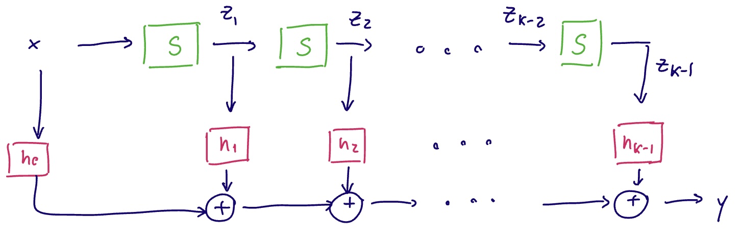
Visual representation of the stepwise local expression

(see convolutional graph filters are local)

Theorem

graph convolution are shift equivariant.

Let $y = H (S) x$ where $S$ is a shift operator. Suppose $x^{'} = S x$ . To show shift equivariance, we need to show $y^{'} = S y$ (ie the output is shifted in the same way the input was).

Proof

$\begin{aligned} y^{'} = H (S) x^{'} & = \sum_{k = 0}^{K - 1} h_{k} S^{k} (S x) \\ = \sum_{k = 0}^{K - 1} h_{k} S^{k + 1} x \\ = S \sum_{k = 0}^{K - 1} h_{k} S^{k} x \\ = S y \end{aligned}$

(see convolutional graph filters are shift equivariant)

note: if $x$ is shifted/diffused, $y$ is shifted in the same way!

Theorem

graph convolution are permutation equivariant.

Suppose we have a graph shift operator $S$ , a graph signal $x$ , and a permutation matrix $P$ . (recall that $P \in {0, 1}$ such that $P 1 = 1$ , $P 1 = 1$ , $P^{T} P = P P^{T} = I$ ). Suppose we relabel nodes $V = {1, 2, \dots, n}$ according to $P$ , ie, define $S^{'} = P S P^{T}$ and $x^{'} = P x$ . Consider filter $y = H (S) x$ .

Then $y^{'} = H (S) x^{'} = P y$

Proof

$\begin{aligned} y^{'} = H (S^{'}) x^{'} & = \sum_{k = 0}^{K - 1} h_{k} (P S P^{T})^{k} P x \\ = \sum_{k = 0}^{K - 1} h_{k} P S^{k} P^{T} P x \\ = P \sum_{k = 0}^{K - 1} h_{k} S^{k} x \\ = P y \end{aligned}$

Thus $H$ is invariant to permutations. (if $S$ and $x$ are permuted/relabelled, $y$ is relabelled in the same way)

(see convolutional graph filters are permutation equivariant)

1.2 Spectral Representations of Convolutional Graph Filters

This is the fourier transform of a filter.

Given $S = V Λ V^{*}$ , recall that $\hat{x} = G F T (x) = V^{*} x$ is the graph fourier transform and $x = I G F T (x) = V \hat{x}$ (see inverse graph fourier transform)

The graph fourier transform of the filtered signal is given as

\begin{aligned} \hat{y} = V^{*} y & = V^{*} \sum_{k = 0}^{K - 1} h_{k} S^{k} x \\ = V^{*} \sum_{k = 0}^{K - 1} h_{k} S^{k} (V \hat{x}) \\ = \sum_{k = 0}^{K - 1} h_{k} V^{*} (V Λ V^{*})^{V} \hat{x} \\ = \sum_{k = 0}^{K - 1} h_{k} Λ^{k} \hat{x} \end{aligned}

Thus, the GFT of the filter and the operator has the same polynomial relationship, but in the spectral domain.

see spectral representation of a convolutional graph filter

Key Takeaway

in the spectral/frequency domain, we have

\hat{y} = \sum_{k = 0}^{K - 1} h_{k} Λ^{k} \hat{x}

The spectral representation/frequency response of $H (S)$ is

\hat{H (S)} = \sum_{k = 0}^{K - 1} h_{k} Λ^{k}

Observations

the filter is independent from the graph. It is completely defined by the polynomial $h (λ) = \sum_{k = 0}^{K - 1} h_{k} λ^{k}$ in the spectral domain

We can see from above that the filter frequency response only depends on the coefficients for the filter $h_{k}$ and the eigenvalues $Λ$ of the shift operator.
If we consider another graph $\tilde{G}$ with shift operator $\tilde{S}$ and $σ (\tilde{S}) = \tilde{Λ}$ . Then $H (\tilde{S}) = \sum_{k = 0}^{K - 1} h_{k} {\tilde{Λ}}^{k}$

the $i$ th spectral component of output $y$ only depends on $λ_{i}$ and ${\hat{x}}_{i}$

$\hat{H (S)}$ is pointwise in the spectral domain. ie ${\hat{y}}_{i} = \sum_{k = 0}^{K - 1} h_{k} λ_{i}^{k} {\hat{x}}_{i}$ . This follows immediately from the fact that $Λ$ is diagonal.

Idea

The polynomial is fixed once we find the coefficients $h_{k}$ . We can think of $\hat{H (S)}$ as sampling values $λ_{i}$ along the curve $h (λ) = \sum_{k = 0}^{K - 1} h_{k} λ^{k}$ . Thus changing $S$ corresponds to a different set of points sampled from this polynomial.

(see the spectral representation of a graph filter is independent from the graph, the spectral graph filter operates on a signal pointwise)

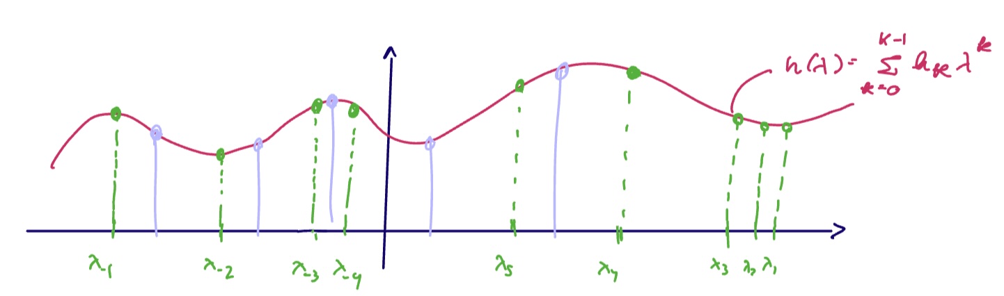
1.2.1 Expressivity of convolutional graph filters

Question

What kinds of functions can $H (S)$ represent (in the spectral domain)?
Suppose we want to design a filter with spectral response $f : R \to R, λ \to f (λ)$ . Can this be implemented as a graph filter?

Answer

Yes, as long as $f$ is analytic - ie, a function with a convergent Taylor series.

see we can represent any analytic function with convolutional graph filters

Fact

Suppose $f$ is an analytic function. Then there exist coefficients $h_{i}$ such that

\begin{aligned} h (λ) & = \sum_{k = 0}^{\infty} h_{k} Λ^{k} \\ = f (0) + λ f^{'} (0) + \frac{λ^{2}}{2!} f^{″} (0) + \frac{λ^{3}}{3!} f^{‴} (0) + \dots \\ = f \end{aligned}

Proof

This follows immediately from the definition of an analytic function

Example

Suppose we have a function $f (λ) = \exp {- \frac{(λ - a)^{2}}{b}}$ . Then $h (λ) = ?$
The Taylor series for $h$ is given as

h (λ) = f (0) + λ f^{'} (0) + \frac{λ^{2}}{2!} f^{″} (0) + \frac{λ^{3}}{3!} f^{‴} (0) + \dots

Here,

$f^{'} = - \frac{2 (λ - a)}{b} \exp {- \frac{(λ - a)^{2}}{b}} ⟹ f^{'} (0) =$
$f^{″} = () ⟹ f^{″} (0) =$
$f^{‴} = ⟹ f^{‴} (0) =$

Thus we can define $H (S) = \sum_{k = 0}^{K - 1} h_{k} Λ^{k}$ with our corresponding coefficients.

Important

We can (and in practice, will) truncate the degree $K$ . This corresponds to the order $K$ Taylor approximation of $f (λ)$ .

Question

What are the limitations of the above expressivity result?

Answer

it is spectral. It does not apply to the graph domain.
This does not account for the specific graph / graph shift operator $S (G)$ or the specific graph signal $x$

In general, we want to answer

Question

Can we use $H (S)$ to represent (or approximate) any signal/representation $y$ ?

Theorem

Let $S$ be a shift operator with eigenvalues $λ_{1}, λ_{2}, \dots, λ_{n}$ , and $x$ a graph signal. Let $\hat{x}$ be the GFT.

Suppose

${\hat{x}}_{i} \neq 0 \forall i$
$λ_{i} \neq λ_{j} \forall i \neq j$

Then there exist $K \leq n$ coefficients $h_{0}, \dots, h_{K - 1}$ such that $y = H (S) x$ .

Proof

Recall from above that

$\hat{y} = h (Λ) \hat{x}$
$\hat{y} = \sum_{k}^{K - 1} h_{k} Λ^{k} \hat{x}$
${\hat{y}}_{i} = \sum_{k}^{K - 1} h_{k} λ_{i}^{k} {\hat{x}}_{i}$

We can write this as a linear system:

\begin{aligned} [\begin{array}{c} {\hat{x}}_{1} & {\hat{x}}_{1} λ_{1} & {\hat{x}}_{1} λ_{1}^{2} & \dots & {\hat{x}}_{1} λ_{1}^{K - 1} \\ {\hat{x}}_{2} & {\hat{x}}_{2} λ_{2} & {\hat{x}}_{2} λ_{2}^{2} & \dots & {\hat{x}}_{2} λ_{2}^{K - 1} \\ ⋮ & ⋮ & ⋮ \\ {\hat{x}}_{n} & {\hat{x}}_{n} λ_{n} & {\hat{x}}_{n} λ_{n}^{2} & \dots & {\hat{x}}_{n} λ_{n}^{K - 1} \end{array}] [\begin{array}{c} h_{0} \\ h_{1} \\ ⋮ \\ h_{K - 1} \end{array}] & = \\ diag (\hat{x}) [\begin{array}{c} 1 & λ_{1} & λ_{1}^{2} & \dots & λ_{1}^{K - 1} \\ 1 & λ_{2} & λ_{2}^{2} & \dots & λ_{2}^{K - 1} \\ ⋮ & ⋮ & ⋮ \\ 1 & λ_{n} & λ_{n}^{2} & \dots & λ_{n}^{K - 1} \end{array}] [\begin{array}{c} h_{0} \\ h_{1} \\ ⋮ \\ h_{K - 1} \end{array}] & = [\begin{array}{c} {\hat{y}}_{1} \\ {\hat{y}}_{2} \\ ⋮ \\ {\hat{y}}_{n} \end{array}] \end{aligned}

Note that LHS $= diag (\hat{x}) V$ where $V$ is a $n \times K$ Vandermonde matrix

In order to find a solution to the system (ie, in order for us to find coefficients $h_{0}, \dots, h_{K - 1}$ ), we need

$diag (\hat{x})$ invertible $⟺ {\hat{x}}_{i} \neq 0 \forall i$
$V h = diag (\hat{x})^{- 1} \hat{y}$ to yield a solution

In the simplest case where $K = n$ , we need the Vandermonde matrix to have an inverse. Since $det (V) = \prod_{i \neq j} (λ_{i} - λ_{j})$ , $V$ is invertible if and only the $λ_{i}$ are distinct.

If $K \neq n$ or arbitrary $K$ , the Rouché-Capelli Theorem states that a linear system with $n$ equations in $K$ unknowns is consistent (ie has a solution) if and only if the rank of the coefficient matrix and the augmented matrix are the same. In this case, this means

\begin{aligned} rank ([\begin{array}{c} 1 & λ_{1} & λ_{1}^{2} & \dots & λ_{1}^{K - 1} \\ 1 & λ_{2} & λ_{2}^{2} & \dots & λ_{2}^{K - 1} \\ ⋮ & ⋮ & ⋮ \\ 1 & λ_{n} & λ_{n}^{2} & \dots & λ_{n}^{K - 1} \end{array}]) & = rank ([\begin{array}{cccccc} 1 & λ_{1} & λ_{1}^{2} & \dots & λ_{1}^{K - 1} & \frac{{\hat{y}}_{1}}{{\hat{x}}_{1}} \\ 1 & λ_{2} & λ_{2}^{2} & \dots & λ_{2}^{K - 1} & \frac{{\hat{y}}_{2}}{{\hat{x}}_{2}} \\ ⋮ & ⋮ & ⋮ & ⋮ \\ 1 & λ_{n} & λ_{n}^{2} & \dots & λ_{n}^{K - 1} & \frac{{\hat{y}}_{n}}{{\hat{x}}_{n}} \end{array}]) \\ ⟸ λ_{i} \neq λ_{j} \forall i \neq j \end{aligned}

(see conditions for finding a convolutional graph filter)